Simple Polynomials of One Variable

8.12

Simple Polynomials of One Variable🔗ℹ

1 A Simple Polynomial Library🔗ℹ

This library provides some basic tools for working with polynomials of one variable.

2 Polynomial Creation, Extraction, and Checking🔗ℹ

(require simple-polynomial/base)
	package: simple-polynomial

procedure
(coefficient? maybe-n) → boolean?
maybe-n : any/c

Determines whether a given value is acceptable as a polynomial coefficient. Racket considers floating point exceptional "numbers" (list +nan.0 +nan.0 +inf.0 -inf.0) as values which qualify as number?s but they will not be accepted as coefficients by this library.

struct
(struct polynomial (terms))
terms : (listof coefficient?)
procedure
(poly coefficient ...) → polynomial?
coefficient : coefficient?

Yields a polynomial with the given coefficients. The leftmost coefficient is the most significant, so for instance

(polynomial '(2 1))

would represent the line 2x+1. The resulting polynomial is a procedure which accepts a single (or/c coefficient? polynomial?) and evaluates the polynomial at that value.

Examples:

> (define P (poly 2 -1 1))
> (P 2)
7

procedure
(poly? p) → boolean?
p : any/c

Short for polynomial?, determines whether the given argument is a polynomial in the sense of this library.

procedure
(poly= p1 p2) → boolean?
p1 : polynomial?
p2 : polynomial?

Equality between two polynomials is determined by agreement on their coefficients.

2.1 Display of Polynomials🔗ℹ

Polynomials are custom printed in a latex-like format, surrounded by greater than and less than symbols, with the variable x, and exponents wrapped in curly-braces, like

"<2x^{2} + 3>"

parameter
(display-short?) → boolean?
(display-short? boolean?) → void?
boolean? : boolean?
= #f

Polynomials in calculations can grow to many terms, so this parameter determines whether polynomials will be shortened for interactive purposes. A shortened polynomial will be truncated in the middle with some ellipses.

Examples:

> (define P (poly 1 2 3 4 5 6 7))
> P
<x^{6} + 2x^{5} + 3x^{4} + 4x^{3} + 5x^{2} + 6x + 7>
> (display-short? #t)
> P
<x^{6} + 2x^{5} + ... + 6x + 7>

procedure
(poly->string p) → string?
p : polynomial?

Converts the given polynomial to a string, exactly as it displays interactively, except that the value of the parameter display-short? is ignored.

procedure
(string->poly s) → polynomial?
s : string?

Interprets a string written in the same format as a polynomial. Although this library will not show coefficients of 1 or exponents of 1, they can be read. Additionally, the "<" and ">" brackets are not required. However, if present all exponents must be wrapped in curly braces. Finally, like terms in the string will be combined.

Examples:

> (define P (poly 1 2 3 4 5 6 7))
> (display-short? #t)
> P
<x^{6} + 2x^{5} + ... + 6x + 7>
> (poly->string P)
"<x^{6} + 2x^{5} + 3x^{4} + 4x^{3} + 5x^{2} + 6x + 7>"
> (string->poly "x+1")
<x + 1>
> (string->poly "x - 2x^{2} + 1 + x + 1")
<-2x^{2} + 2x + 2>

procedure
(poly->latex p [#:inexact-digits id]) → string?
p : polynomial?
id : number? = 4

Converts the given polynomial into a latex-suitable string. If the coefficients of the polynomial are inexact? then #:inexact-digits controls how many digits will print in scientific notation. The output will be mixed between exact? and inexact? representations if the input was mixed.

Examples:

> (define P (poly 1/2 1 1.5 1.334567))
> (poly->latex P)
"\\frac{1}{2}x^{3}+x^{2}+1.5000E0x+1.3346E0"
> (poly->latex P #:inexact-digits 2)
"\\frac{1}{2}x^{3}+x^{2}+1.50E0x+1.33E0"

2.2 Arithmetic🔗ℹ

procedure
(poly+ p ...) → polynomial?
  p : (or/c coefficient? polynomial?)
procedure
(poly- p ...) → polynomial?
  p : (or/c coefficient? polynomial?)
procedure
(poly* p ...) → polynomial?
  p : (or/c coefficient? polynomial?)

Ordinary arithmetic with polynomials. In this library, Racket numbers are interpreted as degenerate polynomials. Each procedure is variadic, which for addition and multiplication is of no consequence since these are commutative operations. Subtraction is then like Racket subtraction, so

(poly- p1 p2 p3)

is like p1 - p2 - p3.

Examples:

> (define p1 (poly 2 -2 12 1))
> (poly+ p1 p1)
<4x^{3} - 4x^{2} + 24x + 2>
> (poly* p1 p1)
<4x^{6} - 8x^{5} + 52x^{4} - 44x^{3} + 140x^{2} + 24x + 1>
> (poly* 2 p1)
<4x^{3} - 4x^{2} + 24x + 2>
> (poly+ 1 1 1)
<3>

procedure
(poly-expt base exponent) → polynomial?
base : polynomial?
exponent : nonnegative-integer?

Repeated multiplication of polynomials.

procedure
(poly-quotient/remainder num den) →
polynomial? polynomial?
num : polynomial?
den : polynomial?

Similar to quotient/remainder, except on polynomials.

procedure
(poly-gcd left right) → polynomial?
left : polynomial?
right : polynomial?

Computes the largest polynomial that divides both left and right with remainder 0.

3 Additional Tools🔗ℹ

(require simple-polynomial/tools)
	package: simple-polynomial

procedure
(points->polynomial pts) → polynomial?
pts : (listof (listof number?))

Takes a list of points, represented as a list or cons of x,y terms, and yields the polynomial determined by these points.

If the desired starting point is not at 0 but at x=a, simply compose the resulting polynomial with (poly 1 (- a)).

procedure
(interpolate-at-integer-points y-values) → polynomial?
y-values : (listof number?)

Like points->polynomial, but assumes x-values are sequential integers starting from 0. Faster than points->polynomial if the points are in this format.

procedure
(rational-roots p) → (listof number?)
p : polynomial?

Finds all rational roots of the given polynomial.

procedure
(falling-factorial n) → polynomial?
n : nonnegative-integer?

Calculates x(x-1)(x-2)...(x-n+1).

procedure
(rising-factorial n) → polynomial?
n : nonnegative-integer?

Calculates x(x+1)(x+2)...(x+n-1).

4 Fitting Points🔗ℹ

(require simple-polynomial/fit)

package: simple-polynomial

A cubic spline would join every pair of points with a cubic equation, and where the cubic equations join at an interior point they would agree on slope and curvature at that joining point. But this still leaves the entire spline underdetermined because the first and last points have no further joins. "Natural" cubic splines set this curvature to zero.

procedure
(points->spline pts) → (listof polynomial?)
pts :
(and/c (listof (listof coefficient?))
(>/c (length pts) 2))

Creates a natural cubic spline for the given points.

procedure
(points->spline-evaluator pts) → procedure?
pts :
(and/c (listof (listof coefficient?))
(>/c (length pts) 2))

Creates an interpolation function from the given points. Some consideration is given to make this evaluation faster for sequential operations like plotting.

Examples:

> (define pts '((1 1) (2 3) (3 -1) (4 1/2)))
> (define peval (points->spline-evaluator pts))
> (peval 1/2)
-59/80
> (peval 0.5)
-0.7374999999999999
> (peval 3)
-1

procedure
(points->best-fit-polynomial pts deg) → polynomial?
pts : (listof (listof coefficient?))
deg : positive-integer?

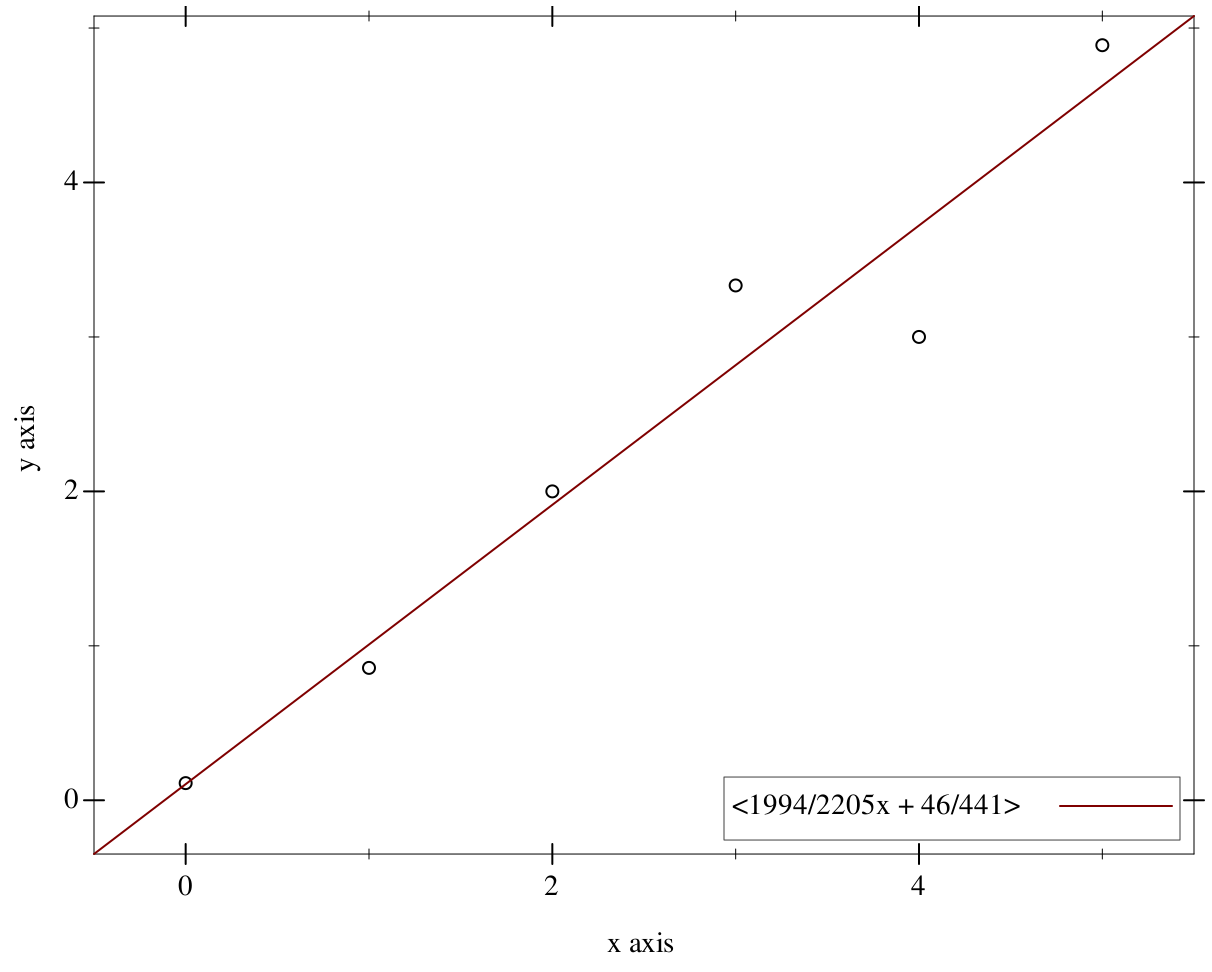
Creates a least-squares approximation polynomial of the given degree. The degree must be at least one larger than the number of points given; if the degree is exactly one more than the number of points given, the fit is exact. If the points can be explained by a polynomial of equal or lesser degree, the fit will be exact.

Examples:

> (define pts (for/list ((x (in-range 6))
                         (noise '(1/9 -1/7 0 1/3 -1 -1/9)))
                (list x (+ x noise))))
> (define P (points->best-fit-polynomial pts 1))
> (plot (list (points pts)
              (function P -0.5 5.5 #:label (poly->string P)))
        #:width 600 #:height 480
        #:legend-anchor 'bottom-right)
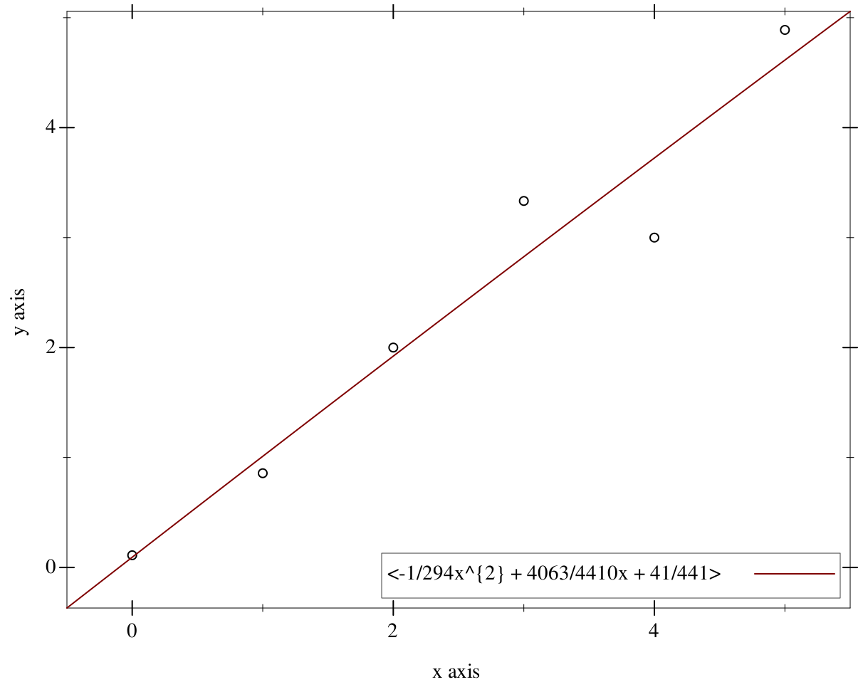
> (define P2 (points->best-fit-polynomial pts 2))
> (plot (list (points pts)
              (function P2 -0.5 5.5 #:label (poly->string P2)))
        #:width 600 #:height 480
        #:legend-anchor 'bottom-right)

For the background of this, see the paper "General Least-Squares Smoothing and Differentiation by the Convolution (Savistzky-Golay) Method". Gorry, P. Anal. Chem. 1990, 62, 570-573.

procedure
(make-least-squares-point-smoother width
order
derivative-order)
→ procedure?
  width : number?
  order : number?
  derivative-order : number?

Produces a function which smooths points based on a moving window of width points. The smoothing function is a least squares polynomial of degree order. A numerical derivative of the points is chosen by derivative-order. The window width should be larger than the number of points to be smoothed by the resulting procedure, and the derivative-order must be greater than or equal to the smoothing order; an argument error will be raised upon application of the resulting procedure if either of these conditions is violated by the points used.

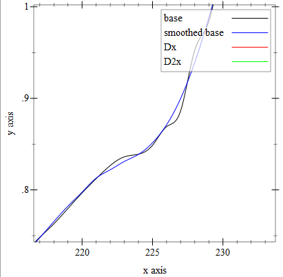
Here is an example image of some real-world data looked at raw, smoothed, and with smoothed first and second order derivatives. 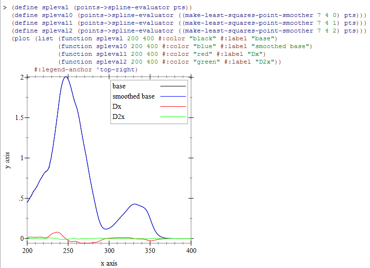The smoothing of the main interpolation is somewhat masked by the scale, so here is a closeup of the unsmoothed and smoothed interpolations.

1	A Simple Polynomial Library
2	Polynomial Creation, Extraction, and Checking
3	Additional Tools
4	Fitting Points