MetaPict

8.12

MetaPict🔗ℹ

Jens Axel Søgaard <jensaxel@soegaard.net>

1 Introduction🔗ℹ

The metapict library provides functions and data structures useful for generating picts. The library includes support for points, vectors, Bezier curves, and, general curves.

The algorithm used to calculate a nice curve from points and tangents is the same as the one used in MetaPost.

With this library I to hope narrow the gap between Scribble and LaTeX + MetaPost/Tikz. If you find any features in MetaPost or Tikz that you miss, don’t hesitate to mail me.

2 Guide🔗ℹ

2.1 Coordinates🔗ℹ

2.1.1 Points🔗ℹ

In order to make a computer draw a shape, a way to specify the key points of the shape is needed.

Note: This is different from racket/pict which reverses the direction of the y-axis.

MetaPict uses standard (x,y)-coordinates for this purpose. The location of a point is always relative to the reference point (0,0). The x-coordinate of a point is the number of units to the right of the reference point. The y-coordinate of a point is the number of units upward from the reference point.

Consider these points:

The coordinates of these points are:

p1=(0,100)		p2=(100,100)		p3=(200,100)
p4=(0,0)		p5=(100,0)		p6=(200,0)

Notice that the point p4=(0,0) is the reference point. The point p3=(200,100) is located 200 units to the right of p4 and 100 units upwards.

In order to write a MetaPict program to draw a shape, a good strategy is to draw the shape on paper. Determine the coordinates for the key points, and then write the MetaPict program that draws lines or curves between the points.

Let us write such a program, that connects point p1 and p6.

> (with-window (window -10 210 -5 105)
(draw (curve (pt 0 100) .. (pt 200 0))))

The .. between the two points connects the two points with a line.

If we are to use the points repeatedly, it is better give them names.

def is shorthand for define

> (def p1 (pt   0 100))
> (def p2 (pt 100 100))
> (def p3 (pt 200 100))
> (def p4 (pt   0   0))
> (def p5 (pt 100   0))
> (def p6 (pt 200   0))
> (with-window (window -10 210 -5 105)
    (draw (curve p1 .. p6)))

Let us connect the point p2 with p5 and p3 with p4.

> (with-window (window -10 210 -5 105)
    (draw (curve p1 .. p6)
          (curve p2 .. p5)
          (curve p3 .. p4)))

If you zoom, you will see that the lines have a thickness and that the ends are rounded. Imagine that you have a pen with a circular nib. The drawings produced by MetaPict will try to mimic the result you get by drawing with such a pen. In the chapter on pens you will learn to the control the thickness of the pen and the shape of the ends of lines.

2.1.2 Displacements🔗ℹ

In the example above, the point p2=(100,100) was described as being 100 to the right and 100 upwards relative to the reference point (0,0).

An alternative way of describing the location of p2 would be to say that is located 100 to the right of p1 (and 0 upwards).

Such a displacement can be described with a vector. Since Racket uses the name "vector", we will represent displacement vectors with a vec structure. To displace a point p with a vector v, use pt+.

> (def v (vec 100 0))
> (def p1 (pt 0 100))
> (def p2 (pt+ p1 v))
> (def p3 (pt+ p2 v))
> (def p4 (pt 0 0))
> (def p5 (pt+ p4 v))
> (def p6 (pt+ p5 v))
> (with-window (window -10 210 -5 105)
    (draw (curve p1 .. p6)
          (curve p2 .. p5)
          (curve p3 .. p4)))

Note: defv is short for define-values.

The point p3 is p1 displaced by v twice. Use vec* to compute 2v. At the same time, let’s use defv to define multiple points at a time.

> (def  v (vec 100 0))
> (def 2v (vec* 2 v))
> (defv (p1 p2 p3) (values (pt 0 100) (pt+ p1 v) (pt+ p1 2v)))
> (defv (p4 p5 p6) (values (pt 0   0) (pt+ p4 v) (pt+ p4 2v)))
> (with-window (window -10 210 -5 105)
    (draw (curve p1 .. p6) (curve p2 .. p5) (curve p3 .. p4)))

The displacements left, right, up, and, down. are predefined. As are the vector operations vec+,vec-, and, vec*. The displacement that moves a point a to point b is given by (pt- b a).

> (list left right up down)
(list (vec -1 0) (vec 1 0) (vec 0 1) (vec 0 -1))
> (vec+ left up)
(vec -1 1)
> (vec- left up)
(vec -1 -1)
> (vec* 3 right)
(vec 3 0)
> (pt- (pt 2 4) (pt 7 8))
(vec -5 -4)

It is common to need points that lie between two point A and B. The mediation operation is called med. The call (med 0.25 A B) will compute the point M on the line from A to B whose distance from A is 25% of the length of AB.

> (def A (pt 0 0))
> (def B (pt 3 2))
> (with-window (window -1 4 -1 3)
    (draw (dot-label "A" A              (top))
          (dot-label "C" (med 0.25 A B) (top))
          (dot-label "D" (med 0.5  A B) (bot))
          (dot-label "E" (med 0.75 A B) (bot))
          (dot-label "B" B              (bot))))

Note: (med x A B) is equivalent to (pt+ A (vec* x (pt- B A))).

Let’s use the knowledge from this section to write a small program to generate the character A. The shape depends on the parameters w (width), h (height) and the placement of the bar α.

> (define (A w h α)
    (set-curve-pict-size w h)
    (def p1 (pt    0    0))
    (def p2 (pt (/ w 2) h))
    (def p3 (pt    w    0))
    (def p4 (med α p1 p2))
    (def p5 (med α p3 p2))
    (with-window (window 0 w 0 h)
      (draw (curve p1 .. p2)
            (curve p2 .. p3)
            (curve p4 .. p5))))
> (list (A 10 20 0.3)
        (A 10 20 0.4)
        (A 10 20 0.5)
        (A 10 20 0.6))
'(   )

3 Reference🔗ℹ

3.1 Points and Vectors (pt and vec)🔗ℹ

(require metapict/pt-vec)

package: metapict

3.1.1 Points and Vectors🔗ℹ

Points and vectors are represented as pt and vec structures respectively. Think of points as positions and of vectors as displacements.

struct
(struct pt (x y)
    #:extra-constructor-name make-pt)
  x : real?
  y : real?

The pt structure represents a point with coordinates (x,y) in the current coordinate system.

> (def A (pt 3 4))
> A
(pt 3 4)
> (pt-x A)
3
> (penwidth 4 (draw (pt 0 0) (pt 1/2 1/2) (pt 1 0)))

struct
(struct vec (x y)
    #:extra-constructor-name make-vec)
  x : real?
  y : real?

The vec structure represents a vector with coordinates (x,y) in the current coordinate system.

> (def v (vec 3 4))
> v
(vec 3 4)
> (vec-x v)
3

3.1.1.1 Predefined Points and Vectors🔗ℹ

The most common points and vectors have predefined names.

value
origo : (pt 0 0)

Origo (0,0) is the reference point of the coordinate system.

value
north : (vec  0  1)
value
south : (vec  0 -1)
value
west : (vec -1  0)
value
east : (vec  1  0)

The compass directions as vecs.

value
up : (vec  0  1)
value
down : (vec  0 -1)
value
left : (vec -1  0)
value
right : (vec  1  0)

Alternative directions names. Note that the direction names make sense only if, the current coordinate system has a positive orientation.

> (penwidth 4 (draw (color "red"     (draw      origo))
                    (color "green"   (draw (pt+ origo north)))
                    (color "blue"    (draw (pt+ origo south)))
                    (color "magenta" (draw (pt+ origo left)))
                    (color "purple"  (draw (pt+ origo right)))))

3.1.1.2 Point Operations🔗ℹ

procedure
(pt+ A v) → pt?
  A : pt?
  v : vec?
(pt+ A B) → pt?
  A : pt?
  B : pt?
(pt+ A B-or-v ...) → pt?
  A : pt
  B-or-v : (or pt? vec?)

Let the coordinates of A, B and v be A=(a1,a2), B=(b1,b2), and, v=(v1,v2).

The form (pt+ A v) returns the displacement of the point A with the vector v. That is, (a1+v1,a2+v2) is returned.

The form (pt+ A B) adds the coordinates of A and B pairwise. The point A is thus displaced with the vector OB. That is, (a1+b1,a2+b2) is returned.

The form (pt+) returns origo, (pt 0 0).

The form (pt+ A) returns the point A.

The form (pt+ A B-or-v ...) returns the result of (pt+ (pt+ A B-or-v) ...).

> (pt+ (pt 1 2) (vec 3 7))
(pt 4 9)
> (pt+ (pt 1 2) (pt 3 7))
(pt 4 9)
> (pt+)
(pt 0 0)
> (pt+ (pt 1 2))
(pt 1 2)
> (pt+ (pt 0.3 0.4) (vec 3 0) (vec 4 0))
(pt 7.3 0.4)

procedure
(pt- A B) → pt?
  A : pt?
  B : pt?
(pt- A v) → pt?
  A : pt?
  v : vec?
(pt- A) → pt?
  A : pt?

The form (pt- B A) returns the vector AB. That is, if A=(a1,a2) and B=(b1,b2), then (b1-a1,b2-a2) is returned.

The form (pt- A v) returns the displacement of the point A with the opposite of vector v. If A=(a1,a2) and v=(v1,v2) then the vector (a1-v1,a2-v2) is returned.

The form (pt- A) returns the reflection of the point A with respect to origo. If A=(a1,a2), then the vector (-a1,-a2) is returned.

> (pt- (pt 1 2) (vec 3 7))
(pt -2 -5)
> (pt- (pt 1 2))
(vec -1 -2)

procedure
(pt* s A) → pt?
s : real?
A : pt?

Scale the coordinates of A with s. If the coordinates of A are (x,y) then the point (sx,sy) is returned.

> (pt* 3 (pt 1 2))
(pt 3 6)

procedure
(dist A B) → real?
A : pt?
B : pt?

Return the distance between the points A and B.

The distance from (x,y) to (a,b) is sqrt((x-a)2 + (y-b)2).

> (dist (pt 4 0) (pt 4 3))
3

procedure
(pt= A B) → boolean?
A : pt?
B : pt?

Returns #t if the coordinates of the point A and B are equal with respect to =. Otherwise #f is returned.

> (pt= (pt 1 2) (pt 1 2))
#t
> (pt= (pt 1 2) (pt 1 42))
#f

procedure
(pt~ A B ε) → boolean?
  A : pt?
  B : pt?
  ε : 1e-15

Returns #t if the distance from the point A to the point is less than or equal to ε. The default value of ε is 1e-15.

> (pt~ (pt 1 2) (pt 1 2.09))
#f
> (pt~ (pt 1 2) (pt 1 2.09) 0.1)
#t

procedure
(med r A B) → pt?
  r : real?
  A : pt?
  B : pt?

The mediate function med computes points between points A and B (if 0<=r<=1). The mediation operation is also known as linear interpolation.

The form (med 1/3 A B) returns the point that lies one-third of the way from A to B.

In general (med r A B) returns the point (1-r)A + rB.

> (def A (pt 0 0))
> (def B (pt 2 1))
> (list (med 0 A B) (med 1/3 A B) (med 1/2 A B) (med 2/3 A B) (med 1 A B))
(list (pt 0 0) (pt 2/3 1/3) (pt 1 1/2) (pt 4/3 2/3) (pt 2 1))
> (set-curve-pict-size 100 50)
> (with-window (window -0.2 2.2 -0.1 1.1)
    (penwidth 4 (draw* (for/list ([r '(0 1/3 1/2 2/3 1)]
                                  [c '("red" "orange" "yellow" "green" "blue")])
                         (color c (draw (med r A B)))))))

procedure
(pt@ r θ) → pt?
r : real?
θ : real?

Returns the point with polar coordinations (r,θ). That is, the point is on the circle with center (0,0) and radius r. The angle from the x-axis to the line through origo and the point is θ. The angle θ is given in radians (0 rad = 0 degrees, π rad = 180 degrees).

> (require racket/math)
> (set-curve-pict-size 50 50)
> (with-window (window -1.1 1.1 -1.1 1.1)
(penwidth 4 (draw* (for/list ([θ (in-range 0 (* 2 pi) (/ (* 2 pi) 12))])
(pt@ 1 θ)))))

procedure
(pt@d r θ) → pt?
r : real?
θ : real?

Same as pt@ but the angle is in degrees.

> (pt@d 1 45)
(pt 0.7071067811865476 0.7071067811865475)
> (pt@ 1 (/ pi 4))
(pt 0.7071067811865476 0.7071067811865475)

3.1.1.3 Vector Operations🔗ℹ

In this section the coordinates of vecs v and w will be referred to as v=(v1,v2) and w=(w1,w2).

procedure
(vec+ v w) → vec?
v : vec?
w : vec?

Returns the vector sum of v and w, that is the vector (v1+w1,v2+w2) is returned.

In terms of displacements the vector sum v+w can be thought of as the result of the displament v followed by the displacement w.

> (def v   (vec 2 0))
> (def w   (vec 0 3))
> (def v+w (vec+ v w))
> v+w
(vec 2 3)
> (define (arrow v [offset (vec 0 0)])
    (def A (pt+ origo offset))
    (draw-arrow (curve A -- (pt+ A v))))
> (ahlength (px 12))
> (with-window (window -0.2 3.2 -0.2 3.2)
    (penwidth 2
      (draw (color "red"   (arrow v))
            (color "green" (arrow w v))
            (color "blue"  (arrow v+w)))))

procedure
(vec- v w) → vec?
v : vec?
w : vec?

Returns the vector difference of v and w, that is the vector (v1-w1,v2-w2) is returned.

procedure
(vec* s v) → vec?
s : real?
v : vec?

Scale the coordinates of v with s. If the coordinates of v are (x,y) then the vector (sx,sy) is returned.

> (vec* 3 (vec 1 2))
(vec 3 6)

procedure
(vec->pt v) → pt?
v : vec?

Converts the vector (x,y) into a point with the same coordinates. If a point A has the same coordinates as a vector v, then the vector is said to a position vector for the point and OA=v.

> (vec->pt (vec 1 2))
(pt 1 2)

procedure
(pos p) → vec?
p : pt?

Converts the point p into a vector with the same coordinates. Such a vector is also called a position vector, hence the name.

> (pos (pt 1 2))
(vec 1 2)

procedure
(vec= v w) → boolean?
v : vec?
w : vec?

Returns #t if the coordinates of the vectors v and w are equal with respect to =. Otherwise #f is returned.

> (vec= (vec 1 2) (vec 1 2))
#t
> (vec= (vec 1 2) (vec 1 42))
#f

procedure
(vec~ v w ε) → boolean?
  v : vec?
  w : vec?
  ε : 1e-15

Returns #t if the length of v-w is less than or equal to ε. The default value of ε is 1e-15.

> (vec~ (vec 1 2) (vec 1 2.09))
#f
> (vec~ (vec 1 2) (vec 1 2.09) 0.1)
#t

procedure
(dot v w) → real?
v : vec?
w : vec?

Returns the dot product of the vectors v and w. The dot product is the number v1 w1 + v2 w2.

The dot product of two vectors are the same as the product of the lengths of the two vectors times the cosine of the angle between the vectors. Thus the dot product of two orthogonal vectors are zero, and the dot product of two vectors sharing directions are the product of their lengths.

> (dot (vec 1 0) (vec 0 1))
0
> (dot (vec 0 2) (vec 0 3))
6

procedure
(len2 v) → real?
v : vec?

Returns the square of the length of the vector v.

> (len2 (vec 1 1))
2
> (len2 (vec 3 4))
25

procedure
(len v) → real?
v : vec?
(norm v) → real?
v : vec?

Returns the length of the vector v.

> (len (vec 1 1))
1.4142135623730951
> (len (vec 3 4))
5

procedure
(dir/rad α) → vec?
α : real?

Returns the unit vector whose angle with the first axis is α radians.

> (dir/rad 0)
(vec 1 0)
> (dir/rad (/ pi 2))
(vec 6.123233995736766e-17 1.0)

procedure
(dir α) → vec?
α : real?

Returns the unit vector whose angle with the first axis is α degrees.

> (dir 0)
(vec 1 0)
> (dir 90)
(vec 6.123233995736766e-17 1.0)

procedure
(vec@ r α) → vec?
r : real?
α : real?

Returns the vector of length r whose angle with the first axis is α radians. In other words construct a vector form polar coordinates.

> (vec@ 2 0)
(vec 2 0)
> (vec@ 2 pi)
(vec -2.0 2.4492935982947064e-16)

procedure
(@ A-or-v) →
real? real?
A-or-v : (or pt? vec?)

Returns the polar coordinates of the point or vector.

> (@ (pt 3 4))
5
0.9272952180016123
> (@ (vec 3 4))
5
0.9272952180016123

procedure
(rot90 A-or-v) → (or pt? vec?)
A-or-v : (or pt? vec?)
(rot-90 A-or-v) → (or pt? vec?)
A-or-v : (or pt? vec?)

Rotates the point or vector 90 or -90 degrees around origo.

> (rot90  (pt  1 0))
(pt 0 1)
> (rot90  (vec 1 0))
(vec 0 1)
> (rot-90 (pt  1 0))
(pt 0 -1)
> (rot-90 (vec 1 0))
(vec 0 -1)

3.2 Colors🔗ℹ

(require metapict/color)

package: metapict

procedure
(make-color* name) → (is-a?/c color%)
  name : string?
(make-color* r g b α) → (is-a?/c color%)
  r : real?
  g : real?
  b : real?
  α : 1.0

The function make-color* is a fault tolerant version of make-color that also accepts color names.

Given a color name as a string, make-color* returns a color% object.

Given real numbers to use as the color components, make-color* works like make-color, but accepts both non-integer numbers, and numbers outside the range 0–255. For a real number x, the value used is (min 255 (max 0 (exact-floor x))).

The optional argument α is the transparency. The default value is 1. Given a transparency outside the interval 0–1, whichever value of 0 and 1 is closest to α is used.

> (def red-ish  (make-color* 300 -12 42.3))
> (def purple   (make-color* "purple"))
> (color->list red-ish)
'(255 0 42 1.0)
> (color->list purple)
'(160 32 240 1.0)
> (with-window (window 0 1 0 1)
    (beside (color red-ish  (fill unitsquare))
            (color purple   (fill unitsquare))))

procedure
(color c p) → pict?
  c : (is-a?/c color%)
  p : pict?
(color f c p) → pict?
  f : real?
  c : (is-a?/c color%)
  p : pict?

In an expression context (color c p) is equivalent to (colorize p c) and (color f c p) is equivalent to (colorize p (color* f c)).

As a match pattern, (color r g b a) matches both color% objects and color names (represented as strings). The variables r, g, and, b will be bound to the red, green, and, blue components of the color. The variable a will be bound to the transparency.

> (with-window (window 0 1 0 1)
    (apply beside (for/list ([f (in-range 0 11/10 1/10)])
                    (color f "red" (fill unitsquare)))))
> (require racket/match)
> (match "magenta"
    [(color r g b a) (list r g b a)])
'(255 0 255 1.0)

procedure
(color->list c) → (listof real?)
c : color

Returns a list of the color components and the transparency of the color c. The color can be a color% object or a color name (string).

> (color->list "magenta")
'(255 0 255 1.0)

procedure
(color+ c1 c2) → (is-a?/c color%)
c1 : color
c2 : color

Returns a color% object, whose color components are the components of c1 and c2 added component-wise. The transparency is (min 1.0 (+ α1 α2)) where α1 and α2 the transparencies of the two colors.

> (color->list (color+ "red" "blue"))
'(255 0 255 1.0)

procedure
(color* k c) → (is-a?/c color%)
k : real?
c : color

Returns a color% object, whose color components are the components of c multiplied component-wise with k. The transparency is the same as in c.

> (color->list (color* 0.5 "blue"))
'(0 0 127 1.0)

procedure
(color-med t c1 c2) → (is-a?/c color%)
  t : real?
  c1 : color
  c2 : color

Interpolates linearly between the colors c1 and c2. For t=0, the color c1 is returned, and when t=1, the color c2 is returned.

> (with-window (window 0 1 0 1)
    (apply beside (for/list ([t (in-range 0 11/10 1/10)])
                    (color (color-med t "red" "yellow")
                           (fill unitsquare)))))

procedure
(color-med* t cs) → (is-a?/c color%)
t : real?
cs : (listof color)

Interpolates linearly between the colors in the list cs. The value "t=0" corresponds to the first color in the list, and "t=1" corresponds to the last color.

> (with-window (window 0 1 0 1)
    (apply beside (for/list ([t (in-range 0 11/10 1/10)])
                    (color (color-med* t '("red" "yellow" "blue" "green"))
                           (fill unitsquare)))))

procedure
(change-red c r) → (is-a?/c color%)
  c : color
  r : real?
procedure
(change-blue c r) → (is-a?/c color%)
  c : color
  r : real?
procedure
(change-green c r) → (is-a?/c color%)
  c : color
  r : real?
procedure
(change-alpha c r) → (is-a?/c color%)
  c : color
  r : real?

Returns a color% object like c where one component has been changed to r.

> (color->list (change-red "blue" 42))
'(42 0 255 1.0)

3.3 Pict🔗ℹ

(require metapict/pict)

package: metapict

3.3.1 Pict Adjusters🔗ℹ

All images in MetaPict are represented as picts. A pict is a structure that holds information on how to draw a picture. A pict can be rendered to produce an image in various formats such as PNG, PDF, and SVG.

The standard library pict defines several functions to construct and manipulate picts. MetaPict provides and offers some extra operations. Since they are not MetaPict specific, they are also useful outside of the world of MetaPict.

A few of the pict operations are provided under new names. The basic concept in MetaPict is the curve. Therefore it makes sense for, say, circle to return a curve. In the pict library the name circle returns a pict, so to avoid a name conflict it is exported as circle-pict.

An attempt has been made to make the pict the last argument of all operations. This explains the existance of a few functions whose functionalities overlap with the pict library.

The operations in this section operate on picts, so use draw to convert curves into picts.

3.3.1.1 Pen Adjusters🔗ℹ

procedure
(color c p) → pict?
c : color?
p : pict?

Draws the pict p with a solid pen and brush of the color c. It is equivalent to (pencolor c (brushcolor c p)).

> (color "red" (filldraw unitcircle))

procedure
(pencolor c p) → pict?
c : color?
p : pict?

Draws the pict p with a solid pen color c. The brush is not affected by pencolor.

> (penwidth 4
(beside (pencolor "red" (brushcolor "orange" (filldraw unitcircle)))
(pencolor "red" (filldraw unitcircle))))

procedure
(penwidth w p) → pict?
w : real?
p : pict?

Draws the pict p with a pen of width w, a real number between 0 and 255. Same as linewidth.

TODO: What unit?!?!

> (apply beside
(for/list ([w 5])
(penwidth w (draw unitcircle))))

procedure
(penscale s p) → pict?
s : real?
p : pict?

Adjusts the current pen width to a width s times wider than the current, then draws the pict p.

> (beside (penwidth 3 (penscale 2 (draw unitcircle)))
(penscale 3 (penwidth 2 (draw unitcircle)))
(penwidth 6 (draw unitcircle)))

procedure
(penstyle s p) → pict?
s : style?
p : pict?

Adjusts the current pen style, and then draws the pict p. The available styles are: 'transparent 'solid 'hilite 'dot 'long-dash 'short-dash 'dot-dash. Note: The pen% documentation mentions a few xor- styles, these are no longer supported by Racket.

> (define (styled-circle style)
    (draw (color "red" (filldraw unitsquare))
          (penstyle style (draw unitcircle))
          (label-bot (~a style) (pt 0 0))))
> (def styles1 '(solid transparent hilite))
> (def styles2 '(dot short-dash long-dash dot-dash))
> (above (beside* (map styled-circle styles1))
         (beside* (map styled-circle styles2)))

procedure
(pencap c p) → pict?
c : cap?
p : pict?

Adjusts the current pen cap, and then draws the pict p. The available caps are: 'round, 'projecting, and, 'butt. The cap determines how the end of curves are drawn. The default pen is 'round.

> (define (squiggle cap)
    (def l (curve (pt -1/2 0) -- (pt 0 0) .. (pt 1/2 1/2)))
    (penwidth 20
      (draw (pencap cap   (color "red"   (draw l)))
            (pencap 'butt (color "black" (draw l)))
            (label-bot (~a cap) (pt 0 -1/2)))))
> (def caps '(round projecting butt))
> (beside* (map squiggle caps))

procedure
(penjoin j p) → pict?
j : join?
p : pict?

Adjusts the current pen join, and then draws the pict p. The available joins are: 'round, 'bevel, and, 'miter. The join determines how the transition from one curve section to the next is drawn. The default join is 'round.

Note: If you want to draw a rectangle with a crisp 90 degree outer angle, then use the 'miter join.

> (define (squiggle join)
    (def l (curve (pt -1/2 0) -- (pt 0 0) .. (pt 1/2 1/2)))
    (draw (penwidth 40 (penjoin join (draw l)))
          (penwidth 2 (color "red" (draw (circle (pt 1/4 -1/3) 1/3))))
          (label-bot (~a join) (pt 0 -1/2))))
> (def joins '(round bevel miter))
> (beside* (map squiggle joins))

procedure
(pen a-pen p) → pict?
a-pen : pen%
p : pict?

Use the pen a-pen as the current pen, then draw the pict p.

> (def teacher-pen
(new pen% [color "red"] [width 1] [style 'solid]
[cap 'round] [join 'round] [stipple #f]))
> (pen teacher-pen (draw unitcircle))

procedure
(dashed p) → pict
p : pict?

Use the pen style 'long-dash to draw the pict p.

> (dashed (draw unitcircle))

procedure
(dotted p) → pict
p : pict?

Use the pen style 'dot to draw the pict p.

> (dotted (draw unitcircle))

3.3.1.2 Brush Adjusters🔗ℹ

procedure
(brush b p) → pict
b : brush%
p : pict?

Use the brush b to draw the pict p.

> (def hatch (new brush% [color "black"] [style 'crossdiag-hatch]))
> (brush hatch (filldraw unitcircle))

procedure
(brushcolor c p) → pict
c : color?
p : pict?

Adjust the brush to use the color b, then draw the pict p.

> (brushcolor "red" (fill unitcircle))

procedure
(brushstyle s p) → pict
s : style?
p : pict?

Adjust the brush to use the style s, then draw the pict p. The example below shows the available styles. The brush style hilite is black with a 30% alpha.

> (define (styled-circle style)
    (draw (color "red" (filldraw (scaled 0.7 unitsquare)))
          (brushcolor "black" (brushstyle style (fill (scaled 0.7 unitcircle))))
          (brushcolor "white" (draw (label-bot (~a style) (pt 0 -0.7))))))
> (def styles1 '(solid transparent hilite))
> (def styles2 '(bdiagonal-hatch fdiagonal-hatch crossdiag-hatch))
> (def styles3 '(horizontal-hatch vertical-hatch cross-hatch))
> (above (beside* (map styled-circle styles1))
         (beside* (map styled-circle styles2))
         (beside* (map styled-circle styles3)))

procedure
(brushstipple s p) → pict
s : style?
p : pict?

Adjust the brush to use the stipple s, then draw the pict p.

> (set-curve-pict-size 256 256)
> (define stipple (bitmap "texture.jpeg"))
> (with-window (window -1 1 -1 1)
    (beside stipple (blank 64 64)
            (brushstipple (pict->bitmap stipple)
                          (fill (circle 1)))))

procedure
(brushgradient TODO:TO-BE-DETERMINED) → pict
TODO:TO-BE-DETERMINED : gradient?

Use a gradient as brush, then draw the pict p.

procedure
(save-pict filename p type) → (void)
  filename : path?
  p : pict?
  type : 'png

Save the pict p as filename. The default format is 'png, other formats include 'svg, 'pdf, 'xbm, 'xpm and 'bmp. JPEG is not included.

procedure
(margin r p) → pict?
r : real?
p : pict?

Equivalent to (inset p r).

3.3.1.3 Pict Combiners🔗ℹ

procedure
(above p ...) → pict?
p : pict?

Draw the picts p ... above each other. If the picts are of different widths, center them.

Same as vc-append

procedure
(beside p ...) → pict?
p : pict?

Draw the picts p ... beside each other. If the picts are of different heights, center them.

Same as hc-append

procedure
(above* ps) → pict?
ps : list?

Draw the picts in the list ps above each other. The first element is on top. If the picts are of different widths, center them.

Same as (apply vc-append ps)

procedure
(beside* ps) → pict?
ps : list?

Draw the picts in the list ps beside each other. The first element is on the left. If the picts are of different heights, center them.

Same as (apply hc-append ps)

3.4 Bezier Curves🔗ℹ

(require metapict/bez)

package: metapict

A Bezier curve from point A to point B with control points A+ and B- is represented as an instance of a bez structure: (bez A A+ B- B).

Graphically such a curve begins at point A and ends at point B. The curve leaves point A directed towards the control point A+. The direction in which the curve enters the end point B is from B-.

The points A and B are referred to as start and end point of the Bezier curve. The points A+ and B- are refererred to as control points. The point A+ is the post control of A and the point B- is the pre control of B.

Most users will not have a reason to work with bez structures directly. The curve constructor is intended to cover all use cases.

Each point on the Bezier curve corresponds to a real number t between 0 and 1. The correspondence is called a parameterization of the curve. The number t is called a parameter. Thus for each value of the parameter t between 0 and 1, you get a point on the curve. The parameter value t=0 corresponds to the start point A and the parameter value t=1 corresponds to the end point.

Let’s see an example of a Bezier curve and its construction.

procedure
(point-of-bez b t) → pt?
b : bez?
t : real?

Return the point on the Bezier curve b that corresponds to the parameter value t. De Casteljau’s algorithm is used to compute the point.

> (def b (bez (pt 0 0) (pt 0 1) (pt 3 2) (pt 5 0)))
> (for/list ([t '(0 1/2 1)])
(point-of-bez b t))
(list (pt 0 0) (pt 7/4 9/8) (pt 5 0))

procedure
(bez~ b1 b2 [ε]) → boolean?
  b1 : bez?
  b2 : bez?
  ε : real? = 0.0001

Returns #t if the defining points of the two Bezier curves are within pairwise distance ε of each other. The default value of ε=0.0001 was chosen to mimic the precision of MetaPost.

> (bez~ (bez (pt 0 0) (pt 0 1) (pt 3 2) (pt 5 0))
(bez (pt 5e-5 0) (pt 0 1) (pt 3 2) (pt 5 0)))
#t

procedure
(bez-reverse b) → bez
b : bez?

Returns a bez representing a Bezier curve whose graph is the same as the graph of the Bezier curve b, but has the reverse orientation.

> (def b     (bez (pt 0 0) (pt 0 1) (pt 3 2) (pt 5 0)))
> (def (γ t) (point-of-bez              b  t))
> (def (φ t) (point-of-bez (bez-reverse b) t))
> (def ts    (in-range 0 5/4 1/4))
> (cons 'γ (for/list ([t ts]) (γ t)))
(list 'γ (pt 0 0) (pt 1/2 45/64) (pt 7/4 9/8) (pt 27/8 63/64) (pt 5 0))
> (cons 'φ (for/list ([t ts]) (φ t)))
(list 'φ (pt 5 0) (pt 27/8 63/64) (pt 7/4 9/8) (pt 1/2 45/64) (pt 0 0))

procedure
(split-bez b t) →
bez? bez?
b : bez?
t : real?

Given a Bezier curve b from p0 to p3 with control points p1 and p2, split the Bezier curve at time t in two parts b1 (from p0 to b(t)) and b2 (from b(t) to p3), such that (point-of-bez b1 1) = (point-of-bez b2 0) and the graphs of b1 and b2 gives the graph of b.

> (def b        (bez (pt 0 0) (pt 0 1) (pt 3 2) (pt 5 0)))
> (defv (b1 b2) (split-bez b 1/3))
> (with-window (window -1 6 -1 6)
    (penwidth 4
      (draw (color "red"  (draw b1))
            (color "blue" (draw b2)))))

procedure
(bez-subpath b t0 t1) → bez?
  b : bez?
  t0 : real?
  t1 : real?

Given a Bezier curve b, return a new Bezier curve c, such that c(0)=b(t0) and c(1)=b(t1) and such that the graph of c is a subset of the graph of b.

> (def b (bez (pt 0 0) (pt 0 1) (pt 3 2) (pt 5 0)))
> (with-window (window -1 6 -1 6)
    (for/draw ([t (in-range 0 5/4 1/4)]
               [c '("red" "blue" "green" "magenta")])
    (penwidth 4
      (beside (draw b)
              (color c (draw (bez-subpath b t (+ t 1/4))))))))

Note: The example shows that the parameterization is not an arc length (aka unit-speed) parameterization.

procedure
(bez-intersection-point b1 b2) → (or pt? #f)
b1 : bez?
b2 : bez?

If the graphs of the Bezier curves intersect, then their first intersection point is returned. If there are no intersections, then #f is returned.

> (def b1 (bez (pt 0.0 0.0) (pt 1.0 1.0) (pt 2.0 2.0) (pt 3.0 3.0)))
> (def b2 (bez (pt 0.0 3.0) (pt 1.0 2.0) (pt 2.0 1.0) (pt 3.0 0.0)))
> (defv (p) (bez-intersection-point b1 b2))
> p
(pt 1.4999999999999996 1.4999999999999996)
> (def b3 (bez (pt 0 4) (pt 1 4) (pt 2 4) (pt 3 4)))
> (bez-intersection-point b1 b3)
#f
> (with-window (window 0 5 0 5)
(draw b1 b2 (color "red" (penwidth 8 (draw p))) b3))

procedure
(bez-intersection-times b1 b2) →
real? real?
b1 : bez?
b2 : bez?

If the graphs of the Bezier curves intersect, numbers t1 and t2 such that b1(t1)=b2(t2) are returned. If there are more than one intersection, the parameter values for the first intersection is returned. If no such numbers exist, the result is (values #f #f).

> (def b1 (bez (pt 0 0) (pt 1 1) (pt 2 2) (pt 3 3)))
> (def b2 (bez (pt 0 3) (pt 1 2) (pt 2 1) (pt 3 0)))
> (defv (t1 t2) (bez-intersection-times b1 b2))
> (defv (p1 p2) (values (point-of-bez b1 t1) (point-of-bez b2 t2)))
> (list p1 p2)
(list
(pt 1.4999999999999998 1.4999999999999998)
(pt 1.4999999999999998 1.5000000000000002))
> (def b3 (bez (pt 0 4) (pt 1 4) (pt 2 4) (pt 3 4)))
> (bez-intersection-times b1 b3)
#f
> (with-window (window 0 5 0 5)
(draw b1 b2 (color "red" (penwidth 8 (draw p1))) b3))

procedure
(bez-intersection-point-and-times b1 b2)
→ (or (list pt? real? real?) #f)
b1 : bez?
b2 : bez?

If the graphs of the Bezier curves intersect, returns a list of the intersection point and two numbers t1 and t2 such that b1(t1)=b2(t2). If there is more than one intersection, the parameter values for the first intersection is returned. If no such numbers exist, the result is (values #f #f).

> (def b1 (bez (pt 0.0 0.0) (pt 1.0 1.0) (pt 2.0 2.0) (pt 3.0 3.0)))
> (def b2 (bez (pt 0.0 3.0) (pt 1.0 2.0) (pt 2.0 1.0) (pt 3.0 0.0)))
> (bez-intersection-point-and-times b1 b2)
(list
(pt 1.4999999999999996 1.4999999999999996)
0.4999999999999999
0.4999999999999999)
> (defm (list p t1 t2) (bez-intersection-point-and-times b1 b2))
> (def b3 (bez (pt 0 4) (pt 1 4) (pt 2 4) (pt 3 4)))
> (bez-intersection-times b1 b3)
#f
> (with-window (window 0 5 0 5)
(draw b1 b2 (color "red" (penwidth 8 (draw p))) b3))

procedure
(draw-bez dc
b
[ #:transformation t
#:pen-transformation pent]) → (void)
  dc : (is-a dc<%>)
  b : bez?
  t : trans? = #f
  pent : trans? = #f

Draws the Bezier curve b on a drawing context dc with optional transformation t and pen-transformation pent.

procedure
(draw-bezs dc
bs
[ #:transformation t
#:pen-transformation pent]) → (void)
  dc : (is-a dc<%>)
  bs : (listof bez?)
  t : trans? = #f
  pent : trans? = #f

Draws the Bezier curves bs on the drawing context dc with optional transformation t and pen-transformation pent.

procedure
(bez->dc-path b [t]) → (is-a? dc<%>)
b : bez?
t : trans? = #f

Convert the Bezier curve b into a dc-path%. If the optional transformation t is present, it is applied to b before the conversion.

procedure
(bezs->dc-path bs [t]) → (is-a? dc<%>)
bs : (listof bez?)
t : trans? = #f

Convert the “consecutive” Bezier curves bs into a dc-path%. If the optional transformation t is present, it is applied to the bs before the conversion.

procedure
(bez/dirs+tensions p0 p3 w0 w3 [τ0 τ3]) → bez?
  p0 : pt?
  p3 : pt?
  w0 : vec?
  w3 : vec?
  τ0 : real? = 1
  τ3 : real? = 1

Returns a bez structure representing a Bezier curve from p0 to p3 that leaves p0 in the direction of w0 and arrives in p3 from the the direction of w0 with tensions t0 and t3, respectively.

> (defv (p0 p3 w0 w3 τ0 τ3) (values (pt 0 0) (pt 5 0) (vec 0 1) (vec 0 -1) 1 1))
> (def b (bez/dirs+tensions p0 p3 w0 w3 τ0 τ3))
> b
(bez
(pt 0 0)
(pt 2.041077998578922e-16 3.333333333333333)
(pt 5.000000000000001 -3.333333333333335)
(pt 5 0))
> (with-window (window -5 11 -5 11) (draw b))

procedure
(control-points p0 p3 θ φ τ0 τ3) → bez?
  p0 : pt?
  p3 : pt
  θ : real?
  φ : real?
  τ0 : real?
  τ3 : real?

Returns a bez structure representing a Bezier curve from p0 to p3 that leaves p0 with an angle of θ and arrives in p3 with an angle of φ with tensions t0 and t3, respectively.

> (defv (p0 p3 θ φ τ0 τ3) (values (pt 0 0) (pt 5 0) pi/2 -pi/2 1 1))
> (defv (p1 p2) (control-points p0 p3 θ φ τ0 τ3))
> (def b (bez p0 p1 p2 p3))
> b
(bez
(pt 0 0)
(pt 2.041077998578922e-16 3.333333333333333)
(pt 5.0 -3.333333333333333)
(pt 5 0))
> (with-window (window -5 11 -5 11) (draw b))

3.5 Curves🔗ℹ

(require metapict/curve)

package: metapict

General curves are drawn by gluing together a series of Bezier curves. Such a curve can be either open or closed (a loop).

The representation of a curve consists simply of a list of Bezier curves and a flag indicating whether the curve is closed. For two consecutive Bezier curves in the list, the end point of the first and the start point of the second must be equal.

The actual representation uses a curve: structure.

struct
(struct curve: (closed? bezs)
    #:extra-constructor-name make-curve:)
  closed? : boolean?
  bezs : (listof bez?)

The reflection name of curve: is 'curve, so the names is printed without the colon suffix.

Most users will not have a reason to work with curve: structures directly. The curve constructor is intended to cover all use cases. The constructor can be used to construct both curved as well as straight lines.

The syntax of curve will be detailed later, but let’s look at some examples. First when multiple points separated by .. are given, a smooth curve through the points will be constructed: (curve p0 .. p1 .. p2 .. p3 .. p4).

As a concrete example, let’s look at the points (0,0) (60,40) (40,90) (10,70) (30,50).

> (def p0 (pt 0   0))
> (def p1 (pt 60 40))
> (def p2 (pt 40 90))
> (def p3 (pt 10 70))
> (def p4 (pt 30 50))
> (define (label-points)
    (for/draw ([i '(0 1 2 3 4)]
               [p (list p0 p1 p2 p3 p4)]
               [d (list (lft) (rt) (top) (lft) (top))])
      (dot-label (~a i) p d)))
> (set-curve-pict-size 120 120)
> (with-window (window -20 100 -20 100)
    (draw (curve p0 .. p1 .. p2 .. p3 .. p4)
          (label-points)))

In order to produce a closed curve, end the curve specification with .. cycle.

> (with-window (window -20 100 -20 100)
(draw (curve p0 .. p1 .. p2 .. p3 .. p4 .. cycle)
(label-points)))

Use -- instead of .. if you want to connect two points with a straight line.

> (with-window (window -20 100 -20 100)
(draw (curve p0 .. p1 .. p2 -- p3 .. p4)
(label-points)))

There is more to the curve constructor (it is possible to specify directions in which a curve enters and leaves a points), but let’s return to operations defined on curves.

The number of Bezier curves used to represent the curve is called the length. The function curve-length returns this length n.

Each point on a curve corresponds to a real number t between 0 and n. The correspondence is called a parameterization of the curve. The number t is called a parameter. Thus for each value of the parameter t between 0 and n, you get a point on the curve. The parameter value t=0 corresponds to the start point A and the parameter value t=n corresponds to the end point.

procedure
(curve-length c) → integer?
c : curve?

Returns the number of Bezier curves used to represent the curve c. This number n is also the end of the interval [0,n] used to parameterize the curve.

> (curve-length (curve p0 .. p1 .. p2 .. p3 .. p4))
4

Given a curve c, one can compute points on the curve corresponding to a parameter value between 0 and the curve length with the function point-of.

procedure
(point-of c t) → pt?
c : curve?
t : real?

Given a curve c and a number t the function point-of computes the point corresponding to the parameter value t. Here, (point-of c 0) and (point-of c (curve-length c)) will return the start and and end point of the curve respectively.

> (let ()
    (define c (curve p0 .. p1 .. p2 .. p3 .. p4))
    (define (label-parameter-values)
      (for/draw ([i '(0 1 2 3 4)]
                 [d (list (lft) (rt) (top) (lft) (top))])
        (define p (point-of c i))
        (dot-label (~a "t=" i) p d)))
    (set-curve-pict-size 120 120)
    (with-window (window -20 100 -20 100)
      (draw c
            (label-parameter-values))))

Since the start and end point of a curve are used often, the following shorthands are available:

procedure
(start-point c) → pt?
c : curve?

Returns the start point of a curve.

procedure
(end-point c) → pt?
c : curve?

Returns the end point of a curve.

> (let ()
(def c (curve (pt 0 0) .. (pt 1 3) .. (pt 2 5)))
(list (start-point c) (end-point c)))
(list (pt 0 0) (pt 2.0 5.0))

Given a curve c parameterized from 0 to n from a start point to an end point, one can use curve-reverse to create a curve where the parameterization is reversed.

procedure
(curve-reverse c) → curve?
c : curve?

Returns a curve through the same points as the curve c. In the parameterization, 0 corresponds to the end point of c and (curve-length c) corresponds to the start point of c.

> (let ()
    (def c (curve (pt 0 0) .. (pt 1 3) .. (pt 2 5)))
    (def r (curve-reverse c))
    (list (start-point c) (end-point c))
    (list (start-point r) (end-point r)))
(list (pt 2 5) (pt 0.0 0.0))

Another way to produce a new curve is to join two existing curves.

procedure
(curve-append c1 c2) → curve?
c1 : curve?
c2 : curve?

Given two curves c1 and c2 where the end point of c1 is the start point of c2, the function curve-append will produce a curve that combines c1 and c2.

> (let ()
    (def c1 (curve (pt 0 0) .. (pt 1 1)))
    (def c2 (curve (pt 1 1) .. (pt 2 0)))
    (def c  (curve-append c1 c2))
    (with-window (window 0 2 0 2)
       (draw (linewidth 6 (color "red"   (draw c1)))
             (linewidth 6 (color "blue"  (draw c2)))
             (linewidth 2 (color "white" (draw c))))))

We will now turn to operations involving two curves. The first problem we will look at is intersections between two curves.

procedure
(intersection-times c1 c2) → (or #f number?)
c1 : curve?
c2 : curve?

If the two curves c1 and c2 have an intersection point, the function will return times (parameter values) t and u such that c1(t)=c2(u). If no intersection point is found, #f is returned.

> (let ()
    (def c1 (curve (pt 0 0) .. (pt 2 3)))
    (def c2 (curve (pt 0 2) .. (pt 4 1)))
    (defv (t u) (intersection-times c1 c2))
    (list (list 't t 'u u)
          (list (point-of c1 t) (point-of c2 u))))
(list
'(t 0.5714285714285715 u 0.2857142857142857)
(list
  (pt 1.1428571428571432 1.7142857142857146)
  (pt 1.1428571428571428 1.7142857142857144)))

procedure
(intersection-point c1 c2) → (or #f pt?)
c1 : curve?
c2 : curve?

Return an intersection point of the curves c1 and c2. If no intersection point exists, the false value #f is returned.

> (let ()
    (def c1 (curve (pt 0 0) .. (pt 2 4)))
    (def c2 (curve (pt 0 4) .. (pt 4 0)))
    (def P  (intersection-point c1 c2))
    (with-window (window 0 4 0 4)
      (draw c1 c2 P (dot-label-rt "P" P))))

If you need both the intersection point and the two times, then fear not:

procedure
(intersection-point-and-times c1 c2)
→ (or #f (list pt? number? number?))
c1 : curve?
c2 : curve?

Return a list (list P t u) where P is an intersection point of the two curves c1 and c2 – and the numbers t and u are times such that P=c1(t)=c2(t).

Finally to get all intersection points of two curves, use intersection-points.

procedure
(intersection-points c1 c2) → (list-of pt?)
c1 : curve?
c2 : curve?

Returns a list of all intersection points of the two curves c1 and c2. If no intersection point exists, the empty list is returned.

> (let ()
    (def c1 (curve (pt 0 0) .. (pt 3 1) .. (pt 2 3) .. (pt 2 1) .. (pt 2.5 1)))
    (def c2 (curve (pt 0 1) .. (pt 1 3) .. (pt 3 0) .. (pt 4 1)))
    (def Ps  (intersection-points c1 c2))
    (with-window (window -1 4 -1 4)
      (draw c1
            (linewidth 2 (color "blue" (draw c2)))
            (color "red" (for/draw ([P Ps])
                           (dot-label "" P (cnt)))))))

If a curve is too long, the function subcurve can be used to make a shorter one.

procedure
(subcurve c t0 t1) → curve?
  c : curve?
  t0 : number?
  t1 : number?

Produces a curve from c(t0) to c(t1). If t0<t1, the direction is reversed.

> (let ()
    (def c (curve (pt 0 0) up .. (pt 1 3) .. (pt 2 0) .. (pt 3 3) .. (pt 3 2)))
    (def s (subcurve c 1 3))
    (with-window (window -1 4 -1 4)
      (draw (linewidth 6 (color "red"   (draw c)))
            (linewidth 2 (color "white" (draw s))))))

Instead of subcurve one can use cut-before and cut-after to make curves shorter.

procedure
(cut-before c1 c2) → curve?
c1 : curve?
c2 : curve?

Cut the part of c1 that lies before the “first” intersection point of the two curves.

> (let ()
    (def c1 (curve (pt 0 0) .. (pt 2 2)))
    (def c2 (curve (pt 0 2) .. (pt 2 0)))
    (def c  (cut-before c1 c2))
    (with-window (window 0 2 0 2)
      (draw (linewidth 6 (color "red"   (draw c1)))
            (linewidth 6 (color "blue"  (draw c2)))
            (linewidth 2 (color "white" (draw c))))))

procedure
(cut-after c1 c2) → curve?
c1 : curve?
c2 : curve?

Cut the part of c1 that lies after the “first” intersection point of the two curves.

> (let ()
    (def c1 (curve (pt 0 0) .. (pt 2 2)))
    (def c2 (curve (pt 0 2) .. (pt 2 0)))
    (def c  (cut-after c1 c2))
    (with-window (window 0 2 0 2)
      (draw (linewidth 6 (color "red"   (draw c1)))
            (linewidth 6 (color "blue"  (draw c2)))
            (linewidth 2 (color "white" (draw c))))))

procedure
(post-control c t) → pt?
c : curve?
t : number?

The curve c consists of a number of Bezier curves. Return the first control point after the parameter value t. See the MetaFontBook page 134.

procedure
(pre-control c t) → pt?
c : curve?
t : number?

The curve c consists of a number of Bezier curves. Return the first control point before the parameter value t. See the MetaFontBook page 134.

procedure
(direction-of c t) → vec?
c : curve?
t : number?

Return the direction in which the curve c is moving at time t.

> (let ()
    (def c (curve (pt 1 0) .. (pt 1 3) .. (pt 4 1)))
    (def p (point-of     c 1))
    (def d (direction-of c 1))
    (with-window (window 0 6 0 6)
      (draw c
            (draw-arrow (curve p .. (pt+ p d)))
            (dot-label-top "P" p))))

procedure
(cyclic? c) → boolean?
c : curve?

Return #t if the curve c is a closed curve.

> (let ()
    (def c1 (curve (pt 1 0) .. (pt 1 3)))
    (def c2 (curve (pt 1 0) .. (pt 1 3) .. cycle))
    (list (cyclic? c1) (cyclic? c2)))
'(#f #t)

procedure
(intercurve α c1 c2) → curve?
  α : number?
  c1 : curve?
  c2 : curve?

Given two curves c1 and c2 of the same length, the call (intercurve α c1 c2) will return a curve “between” the two curves. For α=0 the first curve is returned and for α=1 the second curve is returned.

In other words we can interpolate curves.

> (let ()
    (def heart ; a heart shaped curve
      (curve (pt 100 162) .. (pt 140 178) right .. (pt 195 125) down
             .. (pt 100 0) (curl 0) .. up (pt 5 125) .. right (pt 60 178) .. (pt 100 162)))

    (def fig-heart ; a heart pict
      (with-window (window -100 300 -100 300) (draw heart)))

    (def heart-line ; used to interpolate from line to heart below
      (curve (pt 100 0) -- (pt 300 0) -- (pt 200 0) -- (pt 100 0) -- (pt 0 0)
             -- (pt -100 0) -- (pt 100 0)))

    (def fig-line-to-heart ; shows interpolation between two curves of same length
      (with-window (window -100 300 -100 300)
        (draw* (for/list ([i (in-range 8)])
                 (def α (/ i 8))
                 (color α "red"
                        (draw (intercurve α heart-line heart)))))))

    (beside fig-heart fig-line-to-heart))

procedure
(curve <path-specification-fragment ...) → curve:?
<path-specification-fragment : <path-specification-fragment

The overall purpose of curve is to find a “nice” (possibly closed) curve through a given set of points. If the user wants, they can specify how the curve enters and leaves a point.

Concretely, curve converts a path specification into a list of bezier curves. In the most basic form, a call to curve has one of these forms (but see path operations for more options):

(curve p0 j0 p1 j1 ... pn)

(curve p0 j0 p1 j1 ... pn jn)

(curve p0 j0 p1 j1 ... pn jn cycle)

Here p0, p1, ... are points and j0, j0, ... are path joins. A path join describes how the two points on either side of the path join are to be connected. The most common path joins are .. and --.

> (defv (A B C D) (values (pt -0.3 -0.3) (pt 0.3 -0.3) (pt 0.3 0.3) (pt -0.3 0.3)))
> (let ()
    (beside*
     (list (draw (curve A ..  B ..  C ..  D))
           (draw (curve A --  B --  C --  D))
           (draw (curve A ..  B ..  C ..  D .. cycle))
           (draw (curve A --  B --  C --  D .. cycle)))))

The function curve is a smart constructor, so it accepts a wider range of inputs and rewrites the given path specification into a basic one as the step of computing the list of Bezier curves. In particular, you can use direction specifiers before and/or after a point, to control the direction in which the curve will enter and leave a point.

... j- ds- p ds+ j+ ...

Here the - and + indicates “before” and “after” the point.

Finally curve supports path operations. A path operation f can be placed after a point p:

... p f more ...

In order to process a path specification, curve will make a first pass to remove path operations. When ... p f more ... is encountered, the path operation (a function) f will be called with (list p f more ...) as input. The output is a new path specification where f has been removed.

A few path operations such as /-, -/, --++, -arc, -rectangle are builtin. A user can define their own path operations.

Given two points and a path join (and some extra pieces of information), curve must compute the two control points between the two points.

The standard path joins are .. and --.

value
.. : tension-and? = (tension-and 1 1)
value
-- : full-join? = (full-join (curl 1) .. (curl 1))

Use .. to get “medium bendiness” and -- to get a straight line.

value
cycle : 'cycle

The value used to indicate a closed curve is 'cycle.

struct
(struct join ())
struct
(struct controls-and join (c- c+))
  c- : pt?
  c+ : pt?
struct
(struct tension-and join (τ- τ+))
  τ- : real?
  τ+ : real?
struct
(struct full-join join (ds- j ds+))
  ds- : direction-specifier?
  j : join?
  ds+ : direction-specifier?
procedure
(tension τ) → tension-and?
  τ : real?

These path joins represent the most basic joins. They are not meant to be used directly (although controls-and are occasionally useful), but are used internally.

The “tension” controls how “stiff/bendable” the curve is.

The tension numbers τ- and τ+ are real numbers. If a tension τ is positive, that tension is used. If a tension τ is negative, it is interpreted as “at least abs(τ)”. The default tension is 1. A tension of ∞ gives an (almost) linear curve.

Note: (tension τ) will return (tension-and τ τ), this represents the same tension before and after a point.

> (defv (A B C) (values (pt -0.3 -0.3) (pt -0.3 0.0) (pt 0.3 0.3)))
> (let ()
    (define points (penwidth 4 (color "red" (draw A B C))))
    (beside*
     (list (draw (curve A ..  B (tension  3/4)  C) points)
           (draw (curve A ..  B (tension  1)    C) points)
           (draw (curve A ..  B (tension  2)    C) points)
           (draw (curve A ..  B (tension  3)    C) points)
           (draw (curve A ..  B (tension 10)    C) points))))

The path join controls-and explicitly gives the Bezier control points between the two points. This can be used if a piece of a curve has been computed elsewhere.

> (defv (A B C D) (values (pt -0.3 -0.3) (pt -0.3 0.0) (pt 0.3 0.3) (pt 0.6 0.3)))
> (let ()
    (define points (penwidth 4 (color "red" (draw A B C D))))
    (beside (draw (curve A (controls-and B C) D) points)
            (draw (bez A B C D) points)))

The last basic path join is (full-join ds- j ds+) which allows one to specify an direction ds- for the curve to enter the point and a direction ds+ to leave the points as well as the tension.

A direction specifier can either be empty (represented by #f), an explicit direction (a vec?) or a curl amount.

struct
(struct curl (amount))
amount : real?

Warning: Currently curl doesn’t behave exactly like MetaPost (due to a bug in Metapict).

A join with direction specifiers before and after turns into a full-join.

As an example

... p0 ds0+ j0 ds1- p1 ...

will be rewritten as (full-join ds0+ j0 ds1-).

> (defv (A B C) (values (pt -0.3 -0.3) (pt -0.3 0.0) (pt 0.3 0.3)))
> (let ()
    (define points (penwidth 4 (color "red" (draw A B C))))
    (define (fj v1 v2) (full-join v1 .. v2))
    (beside*
     (list (draw (curve A ..  B (fj (vec  0 1) (vec 1 0)) C) points)
           (draw (curve A ..  B (fj (vec  0 1) (vec 0 1)) C) points)
           (draw (curve A ..  B (fj (vec -1 0) (vec 0 1)) C) points)
           (draw (curve A ..  B (fj (vec -1 0) (vec 1 0)) C) points)
           (draw (curve A ..  B (fj (vec  1 1) (vec 1 1)) C) points))))

> (defv (A B C) (values (pt -0.3 -0.3) (pt -0.3 0.0) (pt 0.3 0.3)))
> (let ()
    (define points (penwidth 4 (color "red" (draw A B C))))
    (define (fj v1 v2) (full-join v1 .. v2))
    (beside*
     (list (draw (curve A ..  B (fj #f (vec 1 0)) C) points)
           (draw (curve A ..  B (fj #f (vec 0 1)) C) points)
           (draw (curve A ..  B (fj #f (vec 0 1)) C) points)
           (draw (curve A ..  B (fj #f (vec 1 0)) C) points)
           (draw (curve A ..  B (fj #f (vec 1 1)) C) points))))

3.6 Transformations🔗ℹ

(require metapict/trans)

package: metapict

Given a curve c, one can use a transformation to calculate a new curve c′ with a different shape or placement. Transformations such as scaling, reflection, rotation and translation appear again and again in graphics programs. These transformations are all affine transformations. An important property of affine transformations is that the composition of two affine transformations is a new affine transformation. If a series of transformations are to be applied to a large set of points or curves, it is more efficient to compute the composed transformation first, and then apply that to the large set.

In MetaPict a transformation can be applied to instances of curve, pt, vec and bez. Furthermore a transformation can be applied to another transformation.

> (def c (curve (pt -1/2 1/2) -- (pt -1/2 0) -- (pt 1/2 0)))
> (penwidth 4
            (draw (color "black" (penwidth 8 (draw c)))
                  (color "red"   (draw ((shifted 1/2 1/2) c)))
                  (color "blue"  (draw ((rotated (/ π 2)) c)))
                  (color "green" (draw (((shifted 0 -0.1) flipy) c)))))

Mathematically an affine transformation transforms a point (x,y) into the point

x′ = ax + cy + e
y′ = bx + dy + f

where a, b, c, d, e and f are real numbers.

struct
(struct trans (a b c d e f)
    #:extra-constructor-name make-trans)
  a : real?
  b : real?
  c : real?
  d : real?
  e : real?
  f : real?

The structure trans represents the affine transformation:

x′ = ax + cy + e
y′ = bx + dy + f

The trans struct is applicable and can be applied to instances of curve, pt, vec and bez. Also a trans can be applied to another trans.

The most used transformations have specialized constructors (see below), so trans is seldom used directly.

> (def t (shifted 10 20))
> (t (pt 1 2))
(pt 11 22)
> (t (vec 1 2))
(vec 11 22)
> (t (curve (pt 1 2) -- (pt 3 4)))
(curve
#f
(list
  (bez
   (pt 11 22)
   (pt 11.666666666666666 22.666666666666668)
   (pt 12.333333333333334 23.333333333333332)
   (pt 13 24))))
> t
(trans 1 0 0 1 10 20)
> (t t)
(trans 1 0 0 1 20 40)
> ((t t) t)
(trans 1 0 0 1 30 60)

value
identity : trans? = (trans 1 0 0 1 0 0)

The identity transformation.

value
rotated90 : trans? = (trans 0 1 -1 0 0 0)

Rotate 90 degrees counterclockwise.

value
rotated180 : trans? = (trans -1 0 0 -1 0 0)

Rotate 180 degrees counterclockwise.

value
rotated270 : trans? = (trans 0 -1 1 0 0 0)

Rotate 270 degrees counterclockwise.

> (def c (curve (pt 0 0) -- (pt 1 0)))
> (penwidth 4
    (draw (color "black" (draw (identity   c)))
          (color "red"   (draw (rotated90  c)))
          (color "blue"  (draw (rotated180 c)))
          (color "green" (draw (rotated270 c)))))

value
flipx : trans? = (trans 1 0 0 -1 0 0)

Reflect about the x-axis.

value
flipy : trans? = (trans -1 0 0 1 0 0)

Reflect about the y-axis.

> (def c (curve (pt 1/4 1/4) -- (pt 1 1)))
> (penwidth 4
    (draw (color "black" (draw (identity c)))
          (color "red"   (draw (flipx    c)))
          (color "blue"  (draw (flipy    c)))))

procedure
(slanted a) → trans?
a : real?

The transformation (trans 1 0 a 1 0 0).

(x,y) slanted a = (x+ay,y)

> (def c (curve (pt 0 0) -- (pt 0 1)))
> (penwidth 4
    (draw (color "black" (draw (identity    c)))
          (color "red"   (draw (slanted 1/3 c)))
          (color "blue"  (draw (slanted 1/2 c)))
          (color "green" (draw (slanted 1   c)))))

procedure
(scaled a) → trans?
a : real?

The transformation (trans a 0 0 a 0 0).

(x,y) scaled a = (ax,ay)

> (def c
    (scaled 1/100
      (shifted -100 -100
          (curve (pt 100 162) .. (pt 140 178) right .. (pt 195 125) down
                 .. (pt 100 0) (curl 0) .. up (pt 5 125)
                 .. right (pt 60 178) .. (pt 100 162)))))
> (penwidth 4
    (draw (color "black" (draw             c))
          (color "red"   (draw (scaled 3/4 c)))
          (color "blue"  (draw (scaled 1/2 c)))
          (color "green" (draw (scaled 1/4 c)))))

procedure
(xscaled a) → trans?
a : real?

The transformation (trans a 0 0 1 0 0).

(x,y) xscaled a = (ax,y)

> (def c
    (scaled 1/100
      (shifted -100 -100
          (curve (pt 100 162) .. (pt 140 178) right .. (pt 195 125) down
                 .. (pt 100 0) (curl 0) .. up (pt 5 125)
                 .. right (pt 60 178) .. (pt 100 162)))))
> (penwidth 4
    (draw (color "black" (draw              c))
          (color "red"   (draw (xscaled 1/2 c)))))

procedure
(yscaled a) → trans?
a : real?

The transformation (trans 1 0 0 a 0 0).

(x,y) yscaled a = (x,ay)

> (def c
    (scaled 1/100
      (shifted -100 -100
          (curve (pt 100 162) .. (pt 140 178) right .. (pt 195 125) down
                 .. (pt 100 0) (curl 0) .. up (pt 5 125)
                 .. right (pt 60 178) .. (pt 100 162)))))
> (penwidth 4
    (draw (color "black" (draw              c))
          (color "red"   (draw (yscaled 1/2 c)))))

procedure
(shifted a b) → trans?
a : real?
b : real?

The transformation (trans 1 0 0 1 a b).

(x,y) yscaled a = (x+a,y+b)

> (def c
    (scaled 1/200
      (shifted -100 -100
          (curve (pt 100 162) .. (pt 140 178) right .. (pt 195 125) down
                 .. (pt 100 0) (curl 0) .. up (pt 5 125)
                 .. right (pt 60 178) .. (pt 100 162)))))
> (penwidth 4
    (draw (color "black" (draw                  c))
          (color "red"   (draw (shifted 1/2 0   c)))
          (color "blue"  (draw (shifted 0   1/2 c)))))

procedure
(zscaled a b) → trans?
a : real?
b : real?

The transformation (trans a b -b a 0 0).

(x,y) zscaled a b = (ax-ay,bx+ay)

Note: (1,0) zscaled (a,b) = (a,b) , thus (1,0) is rotated and scaled into (a,b). Think of zscaled as “complex multiplaction”.

In the example, the red curve is multiplied with 0+1i, which corresponds to a rotation of 90 degrees.

In the example, the blue curve is multiplied with 1+1i, which corresponds to a rotation of 45 degrees. Also, since the magnitude of 1+1i is sqrt(2), the figure is scaled by the factor sqrt(2).

> (def c
    (scaled 1/200
      (shifted -100 -100
          (curve (pt 100 162) .. (pt 140 178) right .. (pt 195 125) down
                 .. (pt 100 0) (curl 0) .. up (pt 5 125)
                 .. right (pt 60 178) .. (pt 100 162)))))
> (penwidth 4
    (draw (color "black" (draw              c))
          (color "red"   (draw (zscaled 0 1 c)))
          (color "blue"  (draw (zscaled 1 1 c)))))

procedure
(rotated θ) → trans?
θ : real?

The transformation (rotated theta) is a rotation of θ radians around (0,0).

> (def c
    (scaled 1/200
      (shifted -100 0
          (curve (pt 100 162) .. (pt 140 178) right .. (pt 195 125) down
                 .. (pt 100 0) (curl 0) .. up (pt 5 125)
                 .. right (pt 60 178) .. (pt 100 162)))))
> (penwidth 4
    (draw (color "black" (draw             c))
          (color "red"   (draw (rotated 3.141592653589793 c)))))

procedure
(rotatedd θ) → trans?
θ : real?

The transformation (rotatedd theta) is a rotation of θ degrees around (0,0).

> (def c
    (scaled 1/200
      (shifted -100 0
          (curve (pt 100 162) .. (pt 140 178) right .. (pt 195 125) down
                 .. (pt 100 0) (curl 0) .. up (pt 5 125)
                 .. right (pt 60 178) .. (pt 100 162)))))
> (penwidth 4
    (draw (color "black" (draw               c))
          (color "red"   (draw (rotatedd 180 c)))))

procedure
(rotated-about θ p) → trans?
θ : real?
p : pt?

The transformation (rotated-about θ) is a rotation of θ radians around the point p.

> (def c
    (scaled 1/200
      (shifted -100 -100
          (curve (pt 100 162) .. (pt 140 178) right .. (pt 195 125) down
                 .. (pt 100 0) (curl 0) .. up (pt 5 125)
                 .. right (pt 60 178) .. (pt 100 162)))))
> (penwidth 4
    (draw (color "black" (draw               c))
          (color "red"   (draw (rotated-about 3.14159 (pt 0.25 0) c)
                                                      (pt 0.25 0)))))

procedure
(rotatedd-about θ p) → trans?
θ : real?
p : pt?

The transformation (rotatedd-about θ p) is a rotation of θ degrees around the point p.

> (def c
    (scaled 1/200
      (shifted -100 -100
          (curve (pt 100 162) .. (pt 140 178) right .. (pt 195 125) down
                 .. (pt 100 0) (curl 0) .. up (pt 5 125)
                 .. right (pt 60 178) .. (pt 100 162)))))
> (penwidth 4
    (draw (color "black" (draw               c))
          (color "red"   (draw (rotatedd-about 180 (pt 0.25 0) c)
                                                   (pt 0.25 0)))
          (color "blue"  (draw (rotatedd-about  90 (pt 0.25 0) c)
                                                   (pt 0.25 0)))))

procedure
(reflected p q) → trans?
p : pt?
q : pt?

The transformation (reflected p q) reflects in the line l through the points p and q.

> (def c
    (scaled 1/200
      (shifted -100 0
          (curve (pt 100 162) .. (pt 140 178) right .. (pt 195 125) down
                 .. (pt 100 0) (curl 0) .. up (pt 5 125)
                 .. right (pt 60 178) .. (pt 100 162)))))
> (draw (curve (pt -1 -1) -- (pt 1 1))
        (penwidth 4
          (draw
           (color "red"   (draw               c))
           (color "blue"  (draw (reflected (pt -1 -1) (pt 1 1) c))))))

procedure
(inverse t) → trans?
t : trans?

If the transformation t is invertible, then (inverse t) is the inverse transformation of t.

> (def c
    (scaled 1/200
      (shifted -100 -100
          (curve (pt 100 162) .. (pt 140 178) right .. (pt 195 125) down
                 .. (pt 100 0) (curl 0) .. up (pt 5 125)
                 .. right (pt 60 178) .. (pt 100 162)))))
> (def t (shifted 1/2 0))
> (def s (inverse t))
> (penwidth 4
    (draw (color "black" (draw c))
          (color "red"   (draw (t c)))
          (color "blue"  (draw (s c)))))

procedure
(trans~ t s [ε]) → boolean?
  t : trans?
  s : trans?
  ε : real? = 1e-15

Compares the two transformations.

> (def t (shifted 1 0))
> (def s (shifted 2 0))
> (trans~ (t t) s)
#t

procedure
(compose-trans t s) → trans?
t : trans?
s : trans?

Compose two transformations. Same as (t s).

procedure
(trans->vector t) → vector?
t : trans?

Compose two transformations. Same as (t s).

> (def t (shifted 42 0))
> (trans->vector t)
'#(1 0 0 1 42 0)

procedure
(trans->transformation t) → vector?
t : trans?

Return a transformation that can be used with the set-transformation method of a drawing context.

> (def t (shifted 42 0))
> (trans->transformation t)
'#(#(1 0 0 1 42 0) 0 0 1 1 0)

3.7 Device Settings🔗ℹ

(require metapict/device)

package: metapict

parameter
(curve-pict-width) → real?
(curve-pict-width width) → void?
width : real?
= 100
parameter
(curve-pict-height) → real?
(curve-pict-height height) → void?
height : real?
= 100

Parameters used to determine the size of the pict created, when a curve is converted into a pict by draw or similar.

The size is in device coordinates.

procedure
(set-curve-pict-size w h) → void?
  w : real?
  h : real?
(set-curve-pict-size p) → void?
  p : pict?

Sets the parameters curve-pict-width and curve-pict-height to w and h or to the width and height of the pict p.

parameter
(curve-pict-window) → window?
(curve-pict-window win) → void?
win : window?
= (window -1.1 1.1 -1.1 1.1)

Parameter that holds the current logical coordinate system in use. The coordinates of points and vectors use the logical coordinate system. When drawn, the logical coordinate system is mapped to device coordinates.

For most purposes, it is practical to keep the aspect ratio of the logical window the same as the device aspect ratio.

procedure
(trans-logical-to-device win
device-width
device-height) → trans?
  win : window
  device-width : real?
  device-height : real?

Computes the affine transformation from the logical coordinate system given by the window win to the window given by (window 0 device-width 0 device-height).

procedure
(current-curve-transformation) → trans?

Computes the transformation from the current window to device coordinates.

procedure
(px a) → real?
  a : real?
procedure
(xpx a) → real?
  a : real?
procedure
(ypx a) → real?
  a : real?

Computes the size of a pixel in logical units.

3.8 Drawing and Filling🔗ℹ

(require metapict/draw)

package: metapict

A curve represents the path of a curve. Use draw and fill to create a picture in the form of a pict. Given a single curve, draw will use the current pen to stroke the path and fill will use the current brush to fill it.

The size of the pict created by draw and fill functions is determined by the parameters curve-pict-width and curve-pict-height.

The position of points, curves etc. are given in logical coordinates. A pict will only draw the section of the coordinate plane that is given by the parameter curve-pict-window. This parameter holds the logical window (an x- and y-range) that will be drawn.

procedure
(draw d ...) → pict?
d : drawable?

Creates a pict representing an image of the drawable arguments.

Given no arguments, a blank pict will be returned.

Given multiple arguments, draw will convert each argument into a pict, then layer the results using cc-superimpose. In other words: it draws the arguments in order, starting with the first.

This table shows how the drawable objects are converted:

curve		curve->pict
pt		draw-dot
bez		bez->pict
label		label->pict
pict		values

> (draw (curve (pt -1 0) .. (pt 0 1) .. (pt 1 0))
        (pt 0 0)
        (bez (pt -1/2 0) (pt -1/2 1) (pt 1/2 1) (pt 1/2 0))
        (label-bot "Origo" (pt 0 0)))

procedure
(draw* ds) → pict?
ds : list?

Draw using draw the non-false values in the list ds on the same pict.

> (penwidth 4
    (draw* (for/list ([n (in-range -5 6)])
             (and (even? n)
                  (pt (/ n 5) (/ n 5))))))

procedure
(fill c ...) → pict?
c : curve?

Creates a pict that uses the current brush to fill either a single curve or to fill areas between curves.

A curve divides the points of the plane in two: the inside and the outside. The inside is drawn with the brush and the outside is left untouched.

For a simple non-intersecting curve it is simple to decide whether a point is on the inside or outside. For self-intersecting curves the so-called winding rule is used. The winding rule is also used when filling multiple curves.

Given a point P, consider a ray from P towards infinity. For each intersection between the ray and the curve(s), determine whether the curve crosses right-to-left or left-to-right. Each right-to-left crossing counts as +1 and each left-to-right crossing as -1. If the total sum of the counts are non-zero, then the point will be filled.

Let’s look at four concentric circles.

> (def circles (map circle '(1 3/4 1/2 1/4)))
> (defm (list c1 c2 c3 c4) circles)

These circles are drawn counter-clockwise. We also need circles that are drawn clockwise:

> (defm (list r1 r2 r3 r4) (map curve-reverse circles))

For a single curve, the orientation doesn’t affect the filling:

> (beside (fill c1) (fill r1))

For the first filled circle, the winding sum is +1, and for the second it is -1. Since they are non-zero, both circles are filled.

The four combinations for two circles are:

> (beside (fill c1 c3)
          (fill c1 r3)
          (fill r1 c3)
          (fill r1 r3))

In the (fill c1 c3) case, the points inside c3 has winding number 2, and inbetween the circles the winding number is +1.

For (fill c1 c3) the winding numbers are -1+1=0 and +1. Therefore the points inside c3 are not filled.

Can you figure out the winding numbers in the these three circle cases?

> (beside (fill c2 r3 c4)
(fill r2 c3 r4))

And for these:

> (beside (fill c1 r2 c3 r4)
(fill r1 c2 r3 c4))

procedure
(eofill c ...) → pict?
c : curve?

Like fill but uses the even-odd rule instead of the winding rule to determine where to fill.

procedure
(filldraw c [fill-color draw-color]) → pict?
  c : curve?
  fill-color : color? = #f
  draw-color : color? = #f

Fill the curve with fill-color, then draw the outline with the color draw-color. If fill-color is #f, then use the brush to fill.

> (penwidth 4 (filldraw unitcircle "darkblue" "purple"))

syntax
(for/draw (for-clause ...) body-or-break ... body)

Iterates like for, but the last expression in the bodys must produce a single drawable value, and the result of the for/draw expression is a pict in which all values are drawn.

> (penwidth 4
(for/draw ([angle (in-range 0 190 10)])
(pt@d 1 angle)))

syntax
(for*/draw (for-clause ...) body-or-break ... body)

Iterates like for*, but the last expression in the bodys must produce a single drawable value, and the result of the for/draw expression is a pict in which all values are drawn.

3.9 Labels🔗ℹ

(require metapict/label)

package: metapict

struct
(struct label (string-or-pict pos plc/vec))
  string-or-pict : string-or-pict?
  pos : pt?
  plc/vec : placement-or-vec?

This struct represents a label. A label is a string or pict, which is drawn next to a certain position pos. The placement of the label in relation to the position is determined by plc/vec.

If plc/vec is the placement top, the label is drawn above the position. The provided placements are: lft, ulft, llft, rt, urt, lrt, top, bot, cnt.

If you need more control over the placment, you can use a vec vektor instead to indicate the direction from pos to the label placement.

struct
(struct placement ())
struct
(struct lft placement ())
struct
(struct ulft placement ())
struct
(struct llft placement ())
struct
(struct rt placement ())
struct
(struct urt placement ())
struct
(struct lrt placement ())
struct
(struct bot placement ())
struct
(struct top placement ())
struct
(struct cnt placement ())

Placements for left, upper left, lower left, right, upper right, lower right, bottom, top and center respectively.

procedure
(label-lft str/pict pos) → label
  str/pict : string-or-pict
  pos : pt?
procedure
(label-ulft str/pict pos) → label
  str/pict : string-or-pict
  pos : pt?
procedure
(label-llft str/pict pos) → label
  str/pict : string-or-pict
  pos : pt?
procedure
(label-rt str/pict pos) → label
  str/pict : string-or-pict
  pos : pt?
procedure
(label-urt str/pict pos) → label
  str/pict : string-or-pict
  pos : pt?
procedure
(label-lrt str/pict pos) → label
  str/pict : string-or-pict
  pos : pt?
procedure
(label-top str/pict pos) → label
  str/pict : string-or-pict
  pos : pt?
procedure
(label-bot str/pict pos) → label
  str/pict : string-or-pict
  pos : pt?
procedure
(label-cnt str/pict pos) → label
  str/pict : string-or-pict
  pos : pt?

Produces a label at position pos where the placement of the label relative to the position is given from the function name.

procedure
(dot-label str/pict pos [plc]) → pict?
  str/pict : string-or-pict?
  pos : pt?
  plc : placement-or-vec? = (bot)

Besides placing the string or pict next to the position pos, also draw a dot at the position.

procedure
(dot-label-lft str/pict pos) → label
  str/pict : string-or-pict
  pos : pt?
procedure
(dot-label-ulft str/pict pos) → label
  str/pict : string-or-pict
  pos : pt?
procedure
(dot-label-llft str/pict pos) → label
  str/pict : string-or-pict
  pos : pt?
procedure
(dot-label-rt str/pict pos) → label
  str/pict : string-or-pict
  pos : pt?
procedure
(dot-label-urt str/pict pos) → label
  str/pict : string-or-pict
  pos : pt?
procedure
(dot-label-lrt str/pict pos) → label
  str/pict : string-or-pict
  pos : pt?
procedure
(dot-label-top str/pict pos) → label
  str/pict : string-or-pict
  pos : pt?
procedure
(dot-label-bot str/pict pos) → label
  str/pict : string-or-pict
  pos : pt?
procedure
(dot-label-cnt str/pict pos) → label
  str/pict : string-or-pict
  pos : pt?

Same as dot-label, but the placement is inferred from the name.

procedure
(label/offset str/pict pos offset) → label?
  str/pict : string-or-pict?
  pos : pt?
  offset : vec?

Like label, but use offset to place the label

procedure
(label-bbox l) → curve?
l : label?

Return a curve along the bounding box of the label l. Useful for debugging label placements.

procedure
(fill-label fill-color l) → pict?
fill-color : color?
l : label?

Fill the bounding box of the label with the fill color, then draw the label. Useful to remove “background noise” below a label.

3.10 Representation🔗ℹ

(require metapict/structs)

package: metapict

This section describes the representation of the MetaPict concepts. The structures have already been described in this manual. The intent is to give an overview of the data structures in a single place.

struct
(struct pt (x y)
    #:extra-constructor-name make-pt)
  x : real?
  y : real?

The pt structure represents a point with coordinates (x,y) in the current coordinate system.

> (def A (pt 3 4))
> A
(pt 3 4)
> (defm (pt x y) A)
> (list x y)
'(3 4)
> (penwidth 4 (draw (pt 0 0) (pt 1/2 1/2) (pt 1 0)))

struct
(struct vec (x y)
    #:extra-constructor-name make-vec)
  x : real?
  y : real?

The vec structure represents a mathematical vector with coordinates (x,y) in the current coordinate system.

> (def v (vec 3 4))
> v
(vec 3 4)
> (defm (vec x y) v)
> (list x y)
'(3 4)
> (def O origo)
> (with-window (window -1 5 -1 5)
(ahlength (px 5))
(draw-arrow (curve O -- (pt+ O v))))

struct
(struct bez (p0 p1 p2 p3)
    #:extra-constructor-name make-bez)
  p0 : pt?
  p1 : pt?
  p2 : pt?
  p3 : pt?

The bez structure represents a cubic Bezier curve with start point in p0, end point in p3 and control points in p1 and p2.

> (with-window (window -1 6 -1 6)
(draw (bez (pt 0 0) (pt 0 1) (pt 2 3) (pt 5 0))))

struct
(struct window (minx maxx miny maxy)
    #:extra-constructor-name make-window)
  minx : real?
  maxx : real?
  miny : real?
  maxy : real?

The window structure represents a rectangular plot window bounded horizontally by minx and maxx and bounded vertically by miny and maxy. By default, the draw command will render a window equivalent to (window -1.1 1.1 -1.1 1.1).

> (draw unitcircle
        (curve (pt 0 1.4) -- (pt 0 0) -- (pt 1.4 0) -- cycle))
> (with-window (window -2 2 -2 2)
    (draw unitcircle
          (curve (pt 0 1.4) -- (pt 0 0) -- (pt 1.4 0) -- cycle)))

4 Examples🔗ℹ

4.1 Rotating Triangle🔗ℹ

This example was inspired by Alain Matthes’s rotated triangle TikZ example.

> (require metapict)
> (def N 18)
> (set-curve-pict-size 300 300)
> (with-window (window -0.1 1.1 -0.1 1.1)
    (defv (A B C) (values (pt 0 0) (pt@d 1 60) (pt 1 0)))
    (first-value
     (for/fold ([drawing (draw)] [A A] [B B] [C C]) ([n N])
       (def triangle (curve A -- B -- C -- cycle))
       (def shade    (color-med (expt (/ n N) 0.4) "red" "yellow"))
       (def filled   (color shade (fill triangle)))
       (values (draw drawing filled triangle)
               (med 0.12 A B) (med 0.12 B C) (med 0.12 C A)))))

4.2 Rooty Helix🔗ℹ

The example shows the lengths of sqrt(n) for values of n from 1 to 86. The design is from Felix Lindemann’s rooty helix TikZ example.

> (require metapict)
> (def max-r 86)
> (def dark-green   (make-color* 175 193 36))
> (def almost-black (make-color*  50  50 50))
> (define (shade r)
    (cond
      [(<= 0 r 1/2) (color-med (* 2 r)         "white"    dark-green)]
      [(<=   r 1)   (color-med (* 2 (- r 1/2)) dark-green almost-black)]
      [else         (error 'shader (~a "got: " r))]))
> (define (spiral drawing max-r)
    (def (node p r)
      (def circ (circle p 1.5))
      (def filled   (color "white" (fill circ)))
      (def label    (label-cnt (~a r) p))
      (draw filled circ label))
    (defv (spiral θ)
      (for/fold ([drawing drawing] [θ 0])
                ([r (in-range 1 max-r)])
        (def √r (sqrt r))
        (def (rotθ c) (scaled 4 (rotated θ c)))
        (defv (A B C) (values (pt 0 0) (rotθ (pt √r 0)) (rotθ (pt √r 1))))
        (def triangle (curve A -- B -- C -- cycle))
        (def filled   (color (shade (/ r 86)) (fill triangle)))
        (values (draw drawing filled triangle (node B r))
                (+ θ (acos (sqrt (/ r (+ 1 r))))))))
    (draw spiral
          (node (scaled 4 (pt@ (sqrt max-r) θ)) max-r)))
> (set-curve-pict-size 600 600)
> (with-window (window -40 40 -40 40)
    (penwidth 0
      (for/fold ([drawing (draw)]) ([r '(86 38 15)])
        (spiral drawing r))))

4.3 Glider - Hacker Emblem🔗ℹ

This figure is a glider, a hacker emblem. The inspiration was Alex Hirzel Glider.

> (set-curve-pict-size 100 100)
> (with-window (window 0 3 0 3)
    (margin 5
      (draw (grid (pt 0 0) (pt 3 3) (pt 0 0) #:step 1)
            (for/draw ([p (list (pt 0 0) (pt 1 0) (pt 2 0) (pt 2 1) (pt 1 2))])
              (color "black" (fill (circle (pt+ p (vec 0.5 0.5)) 0.42)))))))

4.4 Puzzle: The Missing Square🔗ℹ

The two figures are made from the same colored pieces. It seems a square is missing from the bottom figure.

Where is it?

> (define red    (curve (pt 0 0) -- (pt 8 0) -- (pt 8 3) -- cycle))
> (define blue   (curve (pt 0 0) -- (pt 5 0) -- (pt 5 2) -- cycle))
> (define green  (curve (pt 0 0) -- (pt 5 0) -- (pt 5 2) -- (pt 2 2) -- (pt 2 1) -- (pt 0 1) -- cycle))
> (define yellow (curve (pt 0 0) -- (pt 2 0) -- (pt 2 1) -- (pt 5 1) -- (pt 5 2) -- (pt 0 2) -- cycle))
> (define (draw-pieces positions)
    (for/draw ([p positions]
               [d (list  red   green   yellow   blue)]
               [c (list "red" "green" "yellow" "blue")])
      (def fill-color (change-alpha (color-med 0.2 c "magenta") 0.7))
      (def piece (shifted p d))
      (draw (color fill-color (fill piece))
            piece)))
> (set-curve-pict-size 400 (* 13/15 400))
> (with-window (window -1 14 -1 12)
    (define upper (list (pt 0 0) (pt 8 0) (pt 8 1) (pt 8 3)))
    (define lower (list (pt 5 2) (pt 8 0) (pt 5 0) (pt 0 0)))
    (margin 2 (draw (color "gray" (draw (grid (pt -1 -1) (pt 14 12) (pt 0 0) #:step 1)))
                    (draw-pieces (map (shifted (pt 0 6)) upper))
                    (draw-pieces lower))))

4.5 The Olympic Rings🔗ℹ

The inspiration was Paul Gaborit’s The Olympic Rings.

> (struct ring (center color))
> (define r1 (ring (pt -4  0)   (make-color*   0 129 188)))
> (define r2 (ring (pt -2 -1.8) (make-color* 252 177  49)))
> (define r3 (ring (pt  0  0)   (make-color*  35  34  35)))
> (define r4 (ring (pt  2 -1.8) (make-color*   0 157  87)))
> (define r5 (ring (pt  4  0)   (make-color* 238  50  78)))
> (define (draw-rings . rings)
    (for/draw ([r rings])
      (defm (ring p c) r)
      (def c1 (circle p 1.9))
      (def c2 (circle p 1.5))
      (draw (color c (fill c1 (curve-reverse c2)))
            (penwidth 4 (color "white" (draw c1 c2))))))
> (set-curve-pict-size 200 100)
> (with-window (window -6 6 -4 2)
    (draw (clipped (rectangle (pt -6  2)   (pt 6 -1.0)) (draw-rings r5 r4 r3 r2 r1))
          (clipped (rectangle (pt -6 -0.8) (pt 6 -3.8)) (draw-rings r1 r2 r3 r4 r5))))

4.6 Cuboid🔗ℹ

A cuboid drawn with a two-point vanishing perspective. The inspiration was Florian Lesaint’s Cuboid.

> (require metapict)
> (def p1 (pt -7 1.5))
> (def p2 (pt  8 1.5))
> (def a1 (pt  0  0))
> (def a2 (pt  0 -2))
> (def a3 (med 0.8 p1 a2))
> (def a4 (med 0.8 p1 a1))
> (def a7 (med 0.7 p2 a2))
> (def a8 (med 0.7 p2 a1))
> (def a5 (intersection-point (curve a8 -- p1) (curve a4 -- p2)))
> (def a6 (intersection-point (curve a7 -- p1) (curve a3 -- p2)))
> (def f6 (curve a2 -- a3 -- a6 -- a7 -- cycle))
> (def f3 (curve a3 -- a4 -- a5 -- a6 -- cycle))
> (def f4 (curve a5 -- a6 -- a7 -- a8 -- cycle))
> (def (a i) (vector-ref (vector #f a1 a2 a3 a4 a5 a6 a7 a8) i))
> (set-curve-pict-size 300 240)
> (with-window (window -2 3 -2.5 1.5)
    (draw (for/draw ([f (list f3 f4 f6)]
                     [c (map (λ (x) (color* x "gray")) '(0.9 0.7 0.6))])
            (color c (fill f)))
          (penwidth 2
            (for/draw ([line '((5 6) (3 6) (7 6) (1 2) (3 4) (7 8)
                               (1 4) (1 8) (2 3) (2 7) (4 5) (8 5))])
              (defm (list i j) line)
              (curve (a i) -- (a j))))
          (penwidth 8
            (color "red" (draw a1 a2 a3 a4 a5 a6 a7 a8)))))

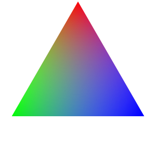
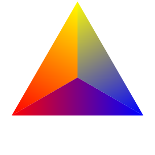
4.7 RGB Triangle🔗ℹ

This example shows how linear gradients can be used to fill a triangle. The first example uses gradients from one color to another along the edge of a triangle. The second example shows how fading from a color c to (change-alpha c 0) is done.

The rgb-triangle was inspired by Andrew Stacey’s RGB Triangle.

> (require file/convertible racket/draw racket/gui)
cannot instantiate `racket/gui/base' a second time in the
same process
> (defv (O A B C) (values (pt 0 0) (pt@d 1 90) (pt@d 1 210) (pt@d 1 330)))
> (with-window (window -1 1 -1 1)
    (def ABC (curve A -- B -- C -- cycle))
    (def (tri P Q c)
      (def g (linear-gradient P Q (list c (change-alpha c 0))))
      (brushgradient g (fill ABC)))
    (draw (tri A (pt@d 1/2 (+  90 180)) "red")
          (tri B (pt@d 1/2 (+ 210 180)) "green")
          (tri C (pt@d 1/2 (- 330 180)) "blue")))
> (with-window (window -1 1 -1 1)
    (def (tri P Q . colors)
      (def g (linear-gradient P Q colors))
      (brushgradient g
        (fill (curve P -- Q -- O -- cycle))))
    (draw (tri A B "yellow" "red")
          (tri B C "red"    "blue")
          (tri C A "blue"   "yellow")))