Graphite: A data visualization library

8.12

Graphite: A data visualization library🔗ℹ

Hazel Levine <hazel@knightsofthelambdacalcul.us>

Graphite is a library designed for producing specific kinds of common graphs/plots, while making decisions about the data being plotted. Graphite is designed to switch between different types of plots relatively seamlessly, without changing anything about the underlying data’s structure.

Graphite is built on top of, and does not replace, plot. For many applications (e.g. 3D plotting, continuous data, interactive plots, etc), plot will be a far better fit.

All of the data-sets that are referred to in this documentation (organdata, oecd, etc) are available here.

A tutorial on graphite is also available; Graphite: a guided tour.

1 Graphing Procedures

1 Graphing Procedures🔗ℹ

procedure
(graph #:data data
#:mapping mapping
[ #:width width
#:height height
#:title title
#:x-label x-label
#:x-transform x-transform
#:x-conv x-conv
#:x-min x-min
#:x-max x-max
#:y-label y-label
#:y-transform y-transform
#:y-conv y-conv
#:y-min y-min
#:y-max y-max
#:facet-wrap facet-wrap
#:legend-anchor legend-anchor
#:theme theme]
renderer ...) → pict?
  data : data-frame?
  mapping : aes?
  width : (or/c rational? #f) = (plot-width)
  height : (or/c rational? #f) = (plot-height)
  title : (or/c string? pict? #f) = (plot-title)
  x-label : (or/c string? pict? #f) = #f
  x-transform : (or/c transform? #f) = #f
  x-conv : (or/c (-> any/c real?) #f) = #f
  x-min : (or/c rational? #f) = #f
  x-max : (or/c rational? #f) = #f
  y-label : (or/c string? pict? #f) = #f
  y-transform : (or/c transform? #f) = #f
  y-conv : (or/c (-> any/c real?) #f) = #f
  y-min : (or/c rational? #f) = #f
  y-max : (or/c rational? #f) = #f
  facet-wrap : (or/c positive-integer? #f) = #f
  legend-anchor : legend-anchor/c = (plot-legend-anchor)
  theme : graphite-theme? = theme-default
  renderer : graphite-renderer?

The primary graphing procedure, producing a pict?. All positional arguments are graphite-renderer?s to be plotted, as returned by points, histogram, et cetera.

The required argument #:data takes a data-frame?, as provided by the data-frame library. Note that the data being fed in must be tidy, meaning that:

Every column is a variable.
Every row is an observation.
Every cell is a single value.

The required argument #:mapping takes a aes? that dictates aesthetics to be applied to every renderer in the specified tree. Generally, you will want at least an x-axis (#:x).

The #:x-conv and #:y-conv arguments, if given, perform pre-processing of the x-axis and y-axis variable (when said variables are not automatically determined). For example, if you wanted to place dates on the x-axis, this could be a function converting your preferred date format to seconds since the UNIX epoch.

The #:x-transform and #:y-transform arguments, if given, take a transform? to adjust the x and y axes, as well as the ticks. For example, if you wanted to place a logarithmic transform on the x-axis, you could specify logarithmic-transform. Transforms are applied after the respective #:x-conv or #:y-conv function, if present.

When given, the #:x-min (etc.) arguments determine the bounds of the plot, but not the bounds of the individual renderers. For this, the data should be trimmed before being passed in.

The aesthetic #:facet, specified in the #:mapping argument, dictates whether to facet on a single categorical variable. If this is selected, Graphite will split the plot into subplots based on that variable, into a grid. This aesthetic will cause unexpected behavior if not applied globally.

The optional #:facet-wrap argument dictates how many columns should be drawn before wrapping to a new line. By default, this is the square root of the number of observations in the #:facet variable, creating a grid.

procedure
(save-pict pict path) → void?
pict : pict?
path : path-string?

Saves a pict? to disk, at the given path. Supports saving as PNG, PDF, or SVG, depending on the file extension.

2 Aesthetic Mappings🔗ℹ

Aesthetic mappings are used to map a given "aesthetic" (such as the x-axis, y-axis, or color) to a variable. When doing this, the given aesthetic will be "split" on that variable. Every renderer, as well as graph, takes an aesthetic mapping using the #:mapping keyword.

procedure
(aes #:<key> value ...) → aes?
value : any/c

Creates an aesthetic mapping, with each #:<key> being mapped to each value.

These objects are generally passed with the #:mapping keyword to either the graph procedure or to each individual graphite-renderer? in the render tree. They dictate various aesthetics, dictating how to display the data (such as colors, variables, et cetera), with behavior being dictated by each renderer.

procedure
(aes? v) → boolean?
v : any/c

Determines if the input is an aesthetic mapping.

procedure
(aes-with/c #:<key> contract ...) → contract?
contract : contract?

Determines if the aesthetic mapping has each #:<key>, with each value satisfying the given contract.

procedure
(aes-containing/c #:<key> contract ...) → contract?
contract : contract?

Determines if the aesthetic mapping optionally contains each #:<key>, and if it does, that each value satisfies the given contract.

3 Renderers🔗ℹ

struct
(struct graphite-renderer (function metadata))
function : (-> (treeof (or/c renderer2d? nonrenderer?)))
metadata : (listof (cons/c parameter? any/c))

The result of each renderer.

Contains both a thunk returning a plot render tree, and an association list of parameters (generally plot parameters) to values, used when a renderer requires certain parameters to be set.

procedure
(points [ #:x-min x-min
#:x-max x-max
#:y-min y-min
#:y-max y-max
#:sym sym
#:color color
#:fill-color fill-color
#:x-jitter x-jitter
#:y-jitter y-jitter
#:size size
#:line-width line-width
#:alpha alpha
#:label label
#:mapping local-mapping]) → graphite-renderer?
  x-min : (or/c rational? #f) = #f
  x-max : (or/c rational? #f) = #f
  y-min : (or/c rational? #f) = #f
  y-max : (or/c rational? #f) = #f
  sym : point-sym/c = (point-sym)
  color : plot-color/c = (point-color)
  fill-color : (or/c plot-color/c 'auto) = 'auto
  x-jitter : (>=/c 0) = (point-x-jitter)
  y-jitter : (>=/c 0) = (point-y-jitter)
  size : (>=/c 0) = (point-size)
  line-width : (>=/c 0) = (point-line-width)
  alpha : (real-in 0 1) = (point-alpha)
  label : (or/c string? pict? #f) = #f
   local-mapping :
(aes-containing/c #:x string?
                  #:y string?
                  #:facet (or/c string? #f)
                  #:discrete-color (or/c string? #f)
                  #:continuous-color (or/c string? #f))
= (aes)

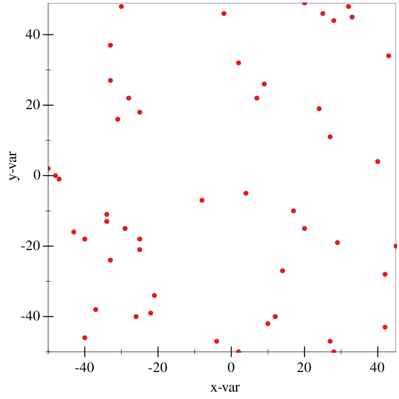
Returns a renderer that draws a set of points, useful for drawing scatterplots or dot-plots. One of the x/y axes (but not both) can be a qualitative variable, in which case a dot-plot is drawn.

Examples:

> (define (random-data)
    (build-vector 50 (λ (_) (random -50 50))))
> (define df (make-data-frame))
> (df-add-series! df (make-series "x-var" #:data (random-data)))
> (df-add-series! df (make-series "y-var" #:data (random-data)))
> (graph #:data df
         #:mapping (aes #:x "x-var" #:y "y-var")
         (points))
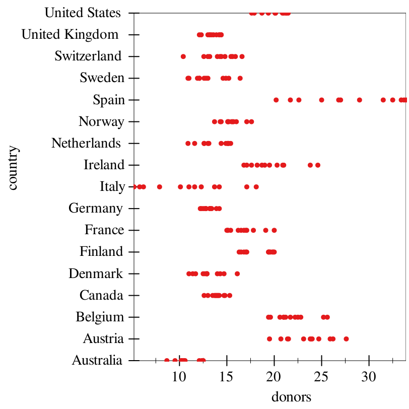
> (graph #:data organdata
         #:mapping (aes #:x "donors" #:y "country")
         (points))

The optional #:discrete-color aesthetic dictates a variable to split on by color, in discrete groups.

Similarly, the #:continuous-color aesthetic dictates a continuous (numeric) variable to split on by color. You likely want to use a continuous colormap (see theme-continuous) for this. Legends for continuous colors are not currently supported. We are working on it.

procedure
(fit [ #:x-min x-min
#:x-max x-max
#:y-min y-min
#:y-max y-max
#:samples samples
#:color color
#:width width
#:style style
#:alpha alpha
#:label label
#:method method
#:span span
#:degree degree
#:show-equation? show-equation?
#:mapping local-mapping]) → graphite-renderer?
  x-min : (or/c rational? #f) = #f
  x-max : (or/c rational? #f) = #f
  y-min : (or/c rational? #f) = #f
  y-max : (or/c rational? #f) = #f
  samples : (and/c exact-integer? (>=/c 2)) = (line-samples)
  color : plot-color/c = (line-color)
  width : (>=/c 0) = (line-width)
  style : plot-pen-style/c = (line-style)
  alpha : (real-in 0 1) = (line-alpha)
  label : (or/c string? pict? #f) = #f
  method : (or/c 'poly 'loess) = 'poly
  span : (real-in 0 1) = span
  degree : positive-integer? = 1
  show-equation? : boolean? = #f
   local-mapping :
(aes-containing/c #:x string?
                  #:y string?
                  #:facet (or/c string? #f))
= (aes)

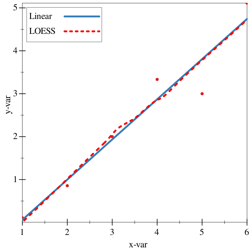
Makes a line of best fit. Internally, this uses the simple-polynomial library’s best fit method for the default 'poly method, or loess for the 'loess method.

Examples:

> (define noise '(1/9 -1/7 0 1/3 -1 1/9))
> (define df (make-data-frame))
> (df-add-series! df (make-series "x-var" #:data (build-vector 6 add1)))
> (df-add-series! df
    (make-series "y-var"
                 #:data (build-vector 6 (λ (x) (+ x (list-ref noise x))))))
> (graph #:data df
         #:mapping (aes #:x "x-var" #:y "y-var")
         (points)
         (fit #:width 3 #:label "Linear")
         (fit #:method 'loess #:color 'red #:style 'dot
              #:width 3 #:label "LOESS"))

The optional #:degree argument specifies the degree of the fit line (2 for a second-degree polynomial, et cetera) in the case of the 'poly method, or the degree of each local fit in the case of 'loess.

See the documentation for loess-fit for details on the #:span parameter.

The optional #:show-equation? argument specifies whether to show the full fit equation in the legend. As LOESS is a non-parametric fit, this requires the 'poly method.

procedure
(lines [ #:x-min x-min
#:x-max x-max
#:y-min y-min
#:y-max y-max
#:color color
#:width width
#:style style
#:alpha alpha
#:label label
#:mapping local-mapping]) → graphite-renderer?
  x-min : (or/c rational? #f) = #f
  x-max : (or/c rational? #f) = #f
  y-min : (or/c rational? #f) = #f
  y-max : (or/c rational? #f) = #f
  color : plot-color/c = (line-color)
  width : (>=/c 0) = (line-width)
  style : plot-pen-style/c = (line-style)
  alpha : (real-in 0 1) = (line-alpha)
  label : (or/c string? pict? #f) = #f
   local-mapping :
(aes-containing/c #:x string?
                  #:y string?
                  #:facet (or/c string? #f)
                  #:discrete-color (or/c string? #f))
= (aes)

Renders some lines connecting the points of the input sequence. This is useful for plotting a time series.

As an example, consider a random walk, adapted from the plot documentation:

> (define df (make-data-frame))
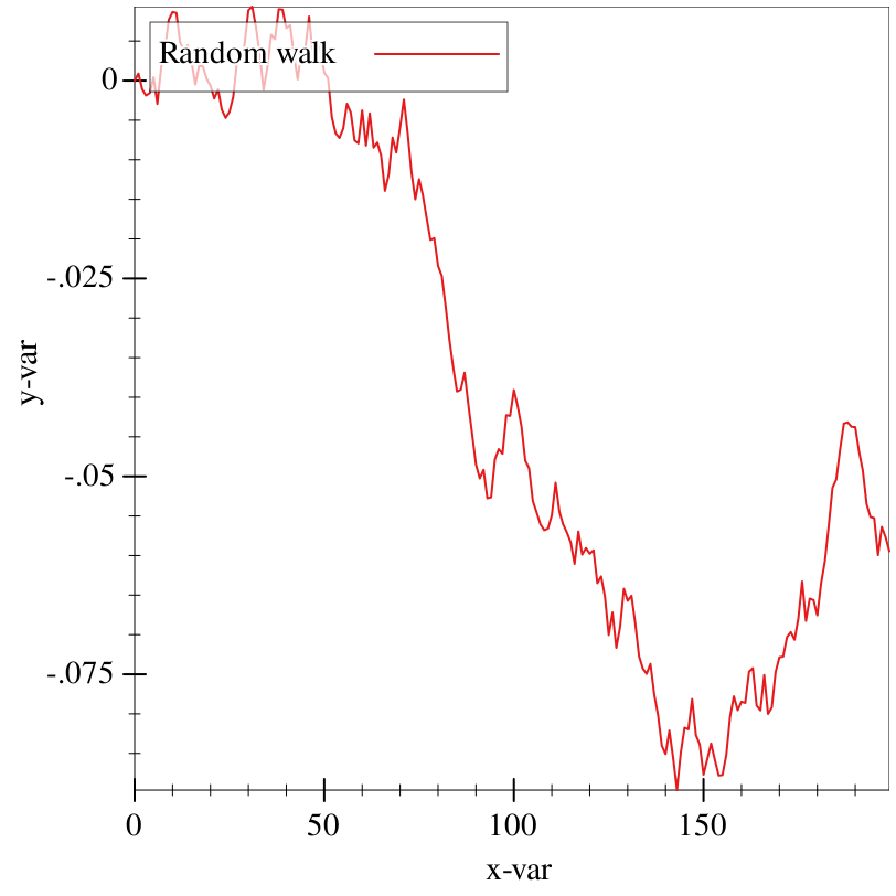
> (define-values (xs ys)
    (for/fold ([xs (list 0)] [ys (list 0)])
              ([i (in-range 1 200)])
      (values (cons i xs) (cons (+ (first ys) (* 1/100 (- (random) 1/2))) ys))))
> (df-add-series! df (make-series "x-var" #:data (list->vector xs)))
> (df-add-series! df (make-series "y-var" #:data (list->vector ys)))
> (graph #:data df
         #:mapping (aes #:x "x-var" #:y "y-var")
         (lines #:label "Random walk"))

procedure
(error-bars #:mapping local-mapping
[ #:x-min x-min
#:x-max x-max
#:y-min y-min
#:y-max y-max
#:color color
#:line-width line-width
#:line-style line-style
#:width width
#:alpha alpha
#:invert? invert?]) → graphite-renderer?
   local-mapping :
(and/c (aes-with/c #:perc-error? string?)
       (aes-containing/c #:x string?
                         #:y string?
                         #:facet (or/c string? #f)))
  x-min : (or/c rational? #f) = #f
  x-max : (or/c rational? #f) = #f
  y-min : (or/c rational? #f) = #f
  y-max : (or/c rational? #f) = #f
  color : plot-color/c = (error-bar-color)
  line-width : (>=/c 0) = (error-bar-line-width)
  line-style : plot-pen-style/c = (error-bar-line-style)
  width : (>=/c 0) = (error-bar-width)
  alpha : (real-in 0 1) = (error-bar-alpha)
  invert? : boolean? = #f

Displays a set of error bars.

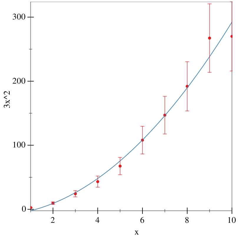
The mandatory aesthetic #:perc-error? dictates the variable in the data-frame that corresponds to percent error. The procedure df-add-derived! may be useful for adding this to a data-frame.

For exmaple, with a constant 20% error:

> (define (3x^2 x) (* 3.0 (expt x 2.0)))
> (define (add-error y) (+ y (* y (/ (- (random 4) 2) 10.0))))
> (define df (make-data-frame))
> (df-add-series! df (make-series "x" #:data (build-vector 10 add1)))
> (df-add-series! df
    (make-series "3x^2"
                  #:data (build-vector 10 (compose add-error 3x^2 add1))))
> (df-add-series! df (make-series "err" #:data (make-vector 10 0.2)))
> (graph #:data df
         #:mapping (aes #:x "x" #:y "3x^2")
         (points)
         (fit #:degree 2)
         (error-bars #:mapping (aes #:perc-error "err")))

procedure
(bar [ #:x-min x-min
#:x-max x-max
#:y-min y-min
#:y-max y-max
#:gap gap
#:skip skip
#:invert? invert?
#:color color
#:style style
#:line-color line-color
#:line-width line-width
#:line-style line-style
#:alpha alpha
#:label label
#:add-ticks? add-ticks?
#:far-ticks? far-ticks?
#:mode mode
#:group-gap group-gap
#:mapping local-mapping]) → graphite-renderer?
  x-min : (or/c rational? #f) = 0
  x-max : (or/c rational? #f) = #f
  y-min : (or/c rational? #f) = 0
  y-max : (or/c rational? #f) = #f
  gap : (real-in 0 1) = (discrete-histogram-gap)
  skip : (>=/c 0) = (discrete-histogram-skip)
  invert? : boolean? = (discrete-histogram-invert?)
  color : plot-color/c = (rectangle-color)
  style : plot-brush-style/c = (rectangle-style)
  line-color : plot-color/c = (rectangle-line-color)
  line-width : (>=/c 0) = (rectangle-line-width)
  line-style : plot-pen-style/c = (rectangle-line-style)
  alpha : (real-in 0 1) = (rectangle-alpha)
  label : (or/c string? pict? #f) = #f
  add-ticks? : boolean? = #t
  far-ticks? : boolean? = #f
  mode : (or/c 'count 'prop) = 'count
  group-gap : (>=/c 0) = 1
   local-mapping :
(aes-containing/c #:x string?
                  #:facet (or/c string? #f)
                  #:group (or/c string? #f))
= (aes)

Renders a bar chart, with calculations done on the data before plotting. For plotting literal data as bars, see col.

The #:mode argument dictates whether the y-axis should be the count of observations by the x-axis ('count), or the relative frequency of those observations ('prop).

The optional #:group aesthetic dictates whether the bar should be "dodged", with each bar being broken up into bars based on the group. If this is enabled, the #:group-gap argument dictates the space between each sub-chart.

procedure
(stacked-bar [ #:x-min x-min
#:x-max x-max
#:y-min y-min
#:y-max y-max
#:gap gap
#:skip skip
#:invert? invert?
#:colors colors
#:styles styles
#:line-colors line-colors
#:line-widths line-widths
#:line-styles line-styles
#:alphas alphas
#:labels labels
#:add-ticks? add-ticks?
#:far-ticks? far-ticks?
#:mode mode
#:mapping local-mapping]) → graphite-renderer?
  x-min : (or/c rational? #f) = #f
  x-max : (or/c rational? #f) = #f
  y-min : (or/c rational? #f) = 0
  y-max : (or/c rational? #f) = #f
  gap : (real-in 0 1) = (discrete-histogram-gap)
  skip : (>=/c 0) = (discrete-histogram-skip)
  invert? : boolean? = (discrete-histogram-invert?)
  colors : (plot-colors/c nat/c) = (stacked-histogram-colors)
   styles : (plot-brush-styles/c nat/c)
= (stacked-histogram-styles)
   line-colors : (plot-colors/c nat/c)
= (stacked-histogram-line-colors)
   line-widths : (pen-widths/c nat/c)
= (stacked-histogram-line-widths)
   line-styles : (plot-pen-styles/c nat/c)
= (stacked-histogram-line-styles)
  alphas : (alphas/c nat/c) = (stacked-histogram-alphas)
  labels : (labels/c nat/c) = '(#f)
  add-ticks? : boolean? = #t
  far-ticks? : boolean? = #f
  mode : (or/c 'count 'prop) = 'count
   local-mapping :
(aes-containing/c #:x string?
                  #:facet (or/c string? #f)
                  #:group string?)
= (aes)

Renders a stacked bar chart, stratified by group.

The mandatory #:group aesthetic dictates what variable each bar should be broken up by.

The #:mode argument dictates whether the y-axis should be the count of observations by the x-axis ('count), or the relative frequency of those observations ('prop). 'prop does not make much sense for stacked bar charts (everything is 100% of itself), but it can be useful in some scenarios.

procedure
(col [ #:x-min x-min
#:x-max x-max
#:y-min y-min
#:y-max y-max
#:color color
#:style style
#:line-color line-color
#:line-width line-width
#:line-style line-style
#:alpha alpha
#:label label
#:gap gap
#:baseline baseline
#:mapping local-mapping]) → graphite-renderer?
  x-min : (or/c rational? #f) = #f
  x-max : (or/c rational? #f) = #f
  y-min : (or/c rational? #f) = #f
  y-max : (or/c rational? #f) = #f
  color : plot-color/c = (rectangle-color)
  style : plot-brush-style/c = (rectangle-style)
  line-color : plot-color/c = (rectangle-line-color)
  line-width : (>=/c 0) = (rectangle-line-width)
  line-style : plot-pen-style/c = (rectangle-line-style)
  alpha : (real-in 0 1) = (rectangle-alpha)
  label : (or/c string? pict? #f) = #f
  gap : real? = 0
  baseline : real? = 0
   local-mapping :
(aes-containing/c #:x string?
                  #:y string?
                  #:discrete-color (or/c string? #f)
                  #:facet (or/c string? #f))
= (aes)

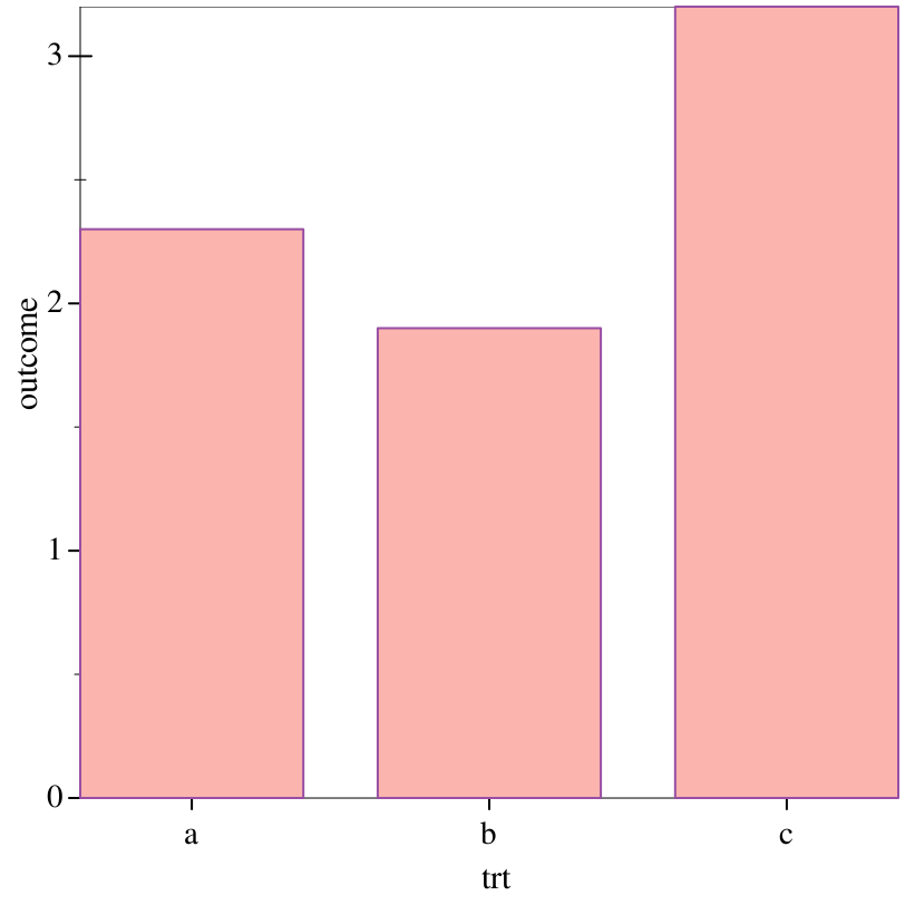
Renders a bar chart. Unlike bar, this treats the specified x and y variables as a collection of variables to be directly displayed, rather than doing further calculations (counting/proportions). The x-axis can be a qualitative variable, but the y-axis must be quantitative.

The optional #:gap argument specifies the gap between each bar.

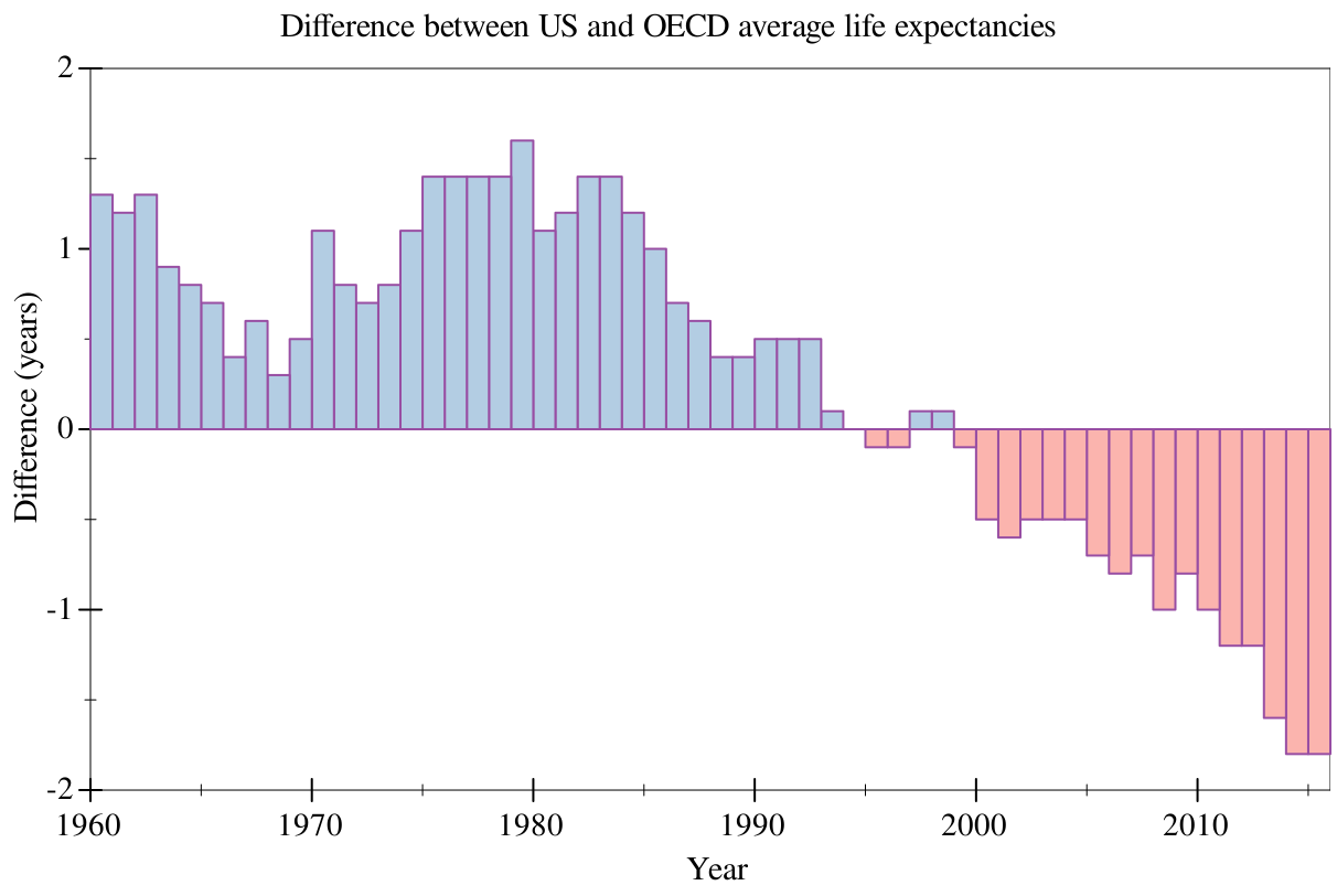
The optional #:baseline argument specifies the baseline of the "x-axis". For example, if you wanted all columns with values above 20 to be above the "x-axis", and all below 20 to be below it, you would set this to be 20.

Examples:

> (define simple (make-data-frame))
> (df-add-series! simple (make-series "trt" #:data (vector "a" "b" "c")))
> (df-add-series! simple (make-series "outcome" #:data (vector 2.3 1.9 3.2)))
> (graph #:data simple
         #:mapping (aes #:x "trt" #:y "outcome")
         (col #:gap 0.25))
> (graph #:data oecd
         #:mapping (aes #:x "year" #:y "diff")
         #:title "Difference between US and OECD average life expectancies"
         #:x-label "Year" #:y-label "Difference (years)"
         #:y-min -2 #:y-max 2
         #:width 600 #:height 400
         #:legend-anchor 'no-legend
         (col #:mapping (aes #:discrete-color "hi_lo")))

procedure
(histogram [ #:x-min x-min
#:x-max x-max
#:y-min y-min
#:y-max y-max
#:color color
#:style style
#:line-color line-color
#:line-width line-width
#:line-style line-style
#:alpha alpha
#:label label
#:bins bins
#:mapping local-mapping]) → graphite-renderer?
  x-min : (or/c rational? #f) = #f
  x-max : (or/c rational? #f) = #f
  y-min : (or/c rational? #f) = #f
  y-max : (or/c rational? #f) = #f
  color : plot-color/c = (rectangle-color)
  style : plot-brush-style/c = (rectangle-style)
  line-color : plot-color/c = (rectangle-line-color)
  line-width : (>=/c 0) = (rectangle-line-width)
  line-style : plot-pen-style/c = (rectangle-line-style)
  alpha : (real-in 0 1) = (rectangle-alpha)
  label : (or/c string? pict? #f) = #f
  bins : positive-integer? = 30
   local-mapping :
(aes-containing/c #:x string?
                  #:y (or/c string? #f)
                  #:facet (or/c string? #f))
= (aes)

Renders a histogram. This is not the same as a bar chart, as the x-axis must be a continuous variable.

The argument #:bins dictates the number of bins on the x-axis.

The optional #:y aesthetic will be the average of every observation in the given x-axis bin. If not specified, this will default to the count of the number of elements in the bin. Anecdotally, if you use this, you may be better off with points or lines.

procedure
(density [ #:x-min x-min
#:x-max x-max
#:y-min y-min
#:y-max y-max
#:samples samples
#:color color
#:width width
#:style style
#:alpha alpha
#:label label
#:mapping local-mapping]) → graphite-renderer?
  x-min : (or/c rational? #f) = #f
  x-max : (or/c rational? #f) = #f
  y-min : (or/c rational? #f) = #f
  y-max : (or/c rational? #f) = #f
  samples : (and/c exact-integer? (>=/c 2)) = (line-samples)
  color : plot-color/c = (line-color)
  width : (>=/c 0) = (line-width)
  style : plot-pen-style/c = (line-style)
  alpha : (real-in 0 1) = (line-alpha)
  label : (or/c string? pict? #f) = #f
   local-mapping :
(aes-containing/c #:x string?
                  #:facet (or/c string? #f)
                  #:discrete-color (or/c string? #f))
= (aes)

Renders estimated density for the given points. The only suppported kernel is the Gaussian, as this is the only supported kernel in plot.

procedure
(boxplot [ #:invert? invert?
#:iqr-scale iqr-scale
#:gap gap
#:box-color box-color
#:box-style box-style
#:box-line-color box-line-color
#:box-line-width box-line-width
#:box-line-style box-line-style
#:box-alpha box-alpha
#:show-outliers? show-outliers?
#:outlier-color outlier-color
#:outlier-sym outlier-sym
#:outlier-fill-color outlier-fill-color
#:outlier-size outlier-size
#:outlier-line-width outlier-line-width
#:outlier-alpha outlier-alpha
#:show-whiskers? show-whiskers?
#:whiskers-color whiskers-color
#:whiskers-width whiskers-width
#:whiskers-style whiskers-style
#:whiskers-alpha whiskers-alpha
#:show-median? show-median?
#:median-color median-color
#:median-width median-width
#:median-style median-style
#:median-alpha median-alpha
#:mapping local-mapping])
→ graphite-renderer?
  invert? : boolean? = #f
  iqr-scale : real? = 1.5
  gap : (real-in 0 1) = (discrete-histogram-gap)
  box-color : plot-color/c = (rectangle-color)
  box-style : plot-brush-style/c = (rectangle-style)
  box-line-color : plot-color/c = (rectangle-line-color)
  box-line-width : (>=/c 0) = (rectangle-line-width)
  box-line-style : plot-pen-style/c = (rectangle-line-style)
  box-alpha : (real-in 0 1) = (rectangle-alpha)
  show-outliers? : boolean? = #t
  outlier-color : plot-color/c = (point-color)
  outlier-sym : point-sym/c = (point-sym)
  outlier-fill-color : (or/c plot-color/c 'auto) = 'auto
  outlier-size : (>=/c 0) = (point-size)
  outlier-line-width : (>=/c 0) = (point-line-width)
  outlier-alpha : (real-in 0 1) = (point-alpha)
  show-whiskers? : boolean? = #t
  whiskers-color : plot-color/c = (line-color)
  whiskers-width : (>=/c 0) = (line-width)
  whiskers-style : plot-pen-style/c = (line-style)
  whiskers-alpha : (real-in 0 1) = (line-alpha)
  show-median? : boolean? = #t
  median-color : plot-color/c = (line-color)
  median-width : (>=/c 0) = (line-width)
  median-style : plot-pen-style/c = (line-style)
  median-alpha : (real-in 0 1) = (line-alpha)
   local-mapping :
(aes-containing/c #:x string?
                  #:y string?
                  #:facet (or/c string? #f))
= (aes)

Renders a box-and-whisker plot. One of the axes (x if not inverted, y if inverted) is assumed to be a qualitative variable.

The optional #:invert? argument, if true, will draw the box-and-whisker plots lengthwise (left-to-right) rather than top-to-bottom. This means that the axes will have to be inverted. For example:

> (graph #:data organdata
         #:mapping (aes #:x "country" #:y "donors")
         (boxplot))
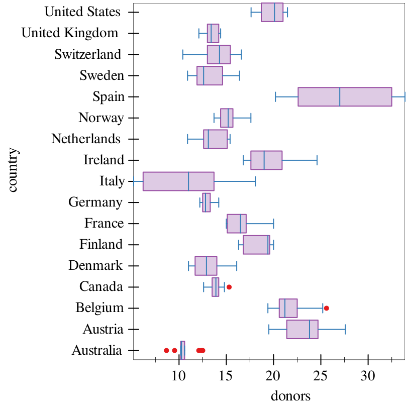
> (graph #:data organdata
         #:mapping (aes #:x "donors" #:y "country")
         (boxplot #:invert? #t))

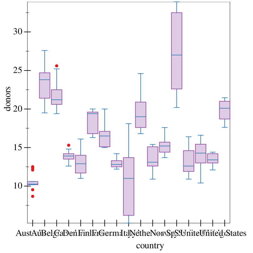
where the second graph is wildly preferable.

The optional #:iqr-scale argument is the multiplier used to determine the lower and upper limits (IQR) and which points are considered arguments. These limits are calculated as (* iqr-scale (- Q3 Q1)), where Q1 and Q3 are (respectively) the first and third quantile of the data.

4 Axis Transforms🔗ℹ

struct
(struct transform (plot-transform axis-ticks))
plot-transform : axis-transform/c
axis-ticks : ticks?

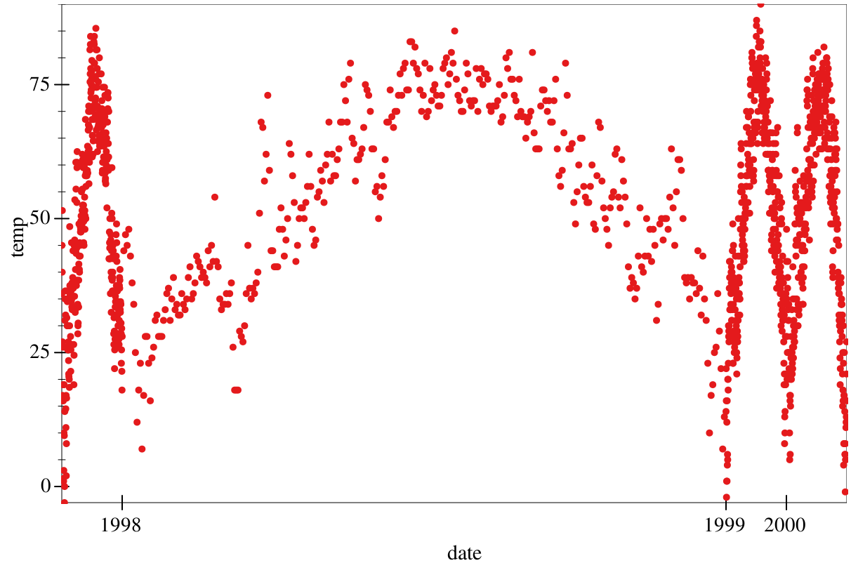
Represents an axis transform, to be used in the #:x-transform or #:y-transform argument of graph.

Takes a plot transform and a ticks? for the respective axis to be applied. For example, to add a stretch transform on an axis where the x-axis is a date:

> (define iso8601->posix (compose ->posix iso8601->date))
> (graph #:data chicago
         #:mapping (aes #:x "date" #:y "temp")
         #:x-transform (transform (stretch-transform
                                   (iso8601->posix "1998-01-01")
                                   (iso8601->posix "1999-01-01")
                                   10)
                                  (date-ticks))
         #:x-conv iso8601->posix
         #:width 600
         (points))

procedure
(get-adjusted-ticks transform) → ticks?
transform : transform?

Gets the adjusted ticks? from the axis transform, for actual usage as plot-x-ticks or plot-y-ticks. Useful both internally and for interoperation with plot.

procedure
(only-ticks ticks) → transform?
ticks : ticks?

Constructs a new transform that only changes the axis ticks according to the input ticks, without actually manipulating the data.

value
no-transform : transform?

The dummy axis transform. Does not manipulate the data.

value
logarithmic-transform : transform?

A logarithmic (base 10) axis transform.

5 Theming🔗ℹ

struct
(struct graphite-theme ( foreground
foreground-alpha
background
background-alpha
font-size
font-face
font-family
pen-color-map
brush-color-map))
  foreground : plot-color/c
  foreground-alpha : (real-in 0 1)
  background : plot-color/c
  background-alpha : (real-in 0 1)
  font-size : (>=/c 0)
  font-face : (or/c string? #f)
  font-family : font-family/c
  pen-color-map : (or/c symbol? #f)
  brush-color-map : (or/c symbol? #f)

Represents a theme, to be passed by the #:theme argument to graph.

These fields correspond to, respectively, the plot parameters plot-foreground, plot-foreground-alpha, plot-background, plot-background-alpha, plot-font-size, plot-font-face, plot-font-family, plot-pen-color-map, and plot-brush-color-map. They correspond to the same behaviors in plot.

The pen-color-map field corresponds to the color-map used to draw points and lines, such as that in points or lines. The brush-color-map field corresponds to the color-map used to draw rectangles and other large fields, such as histogram and bar.

procedure
(make-graphite-theme [ #:fg fg
#:fg-alpha fg-alpha
#:bg bg
#:bg-alpha bg-alpha
#:font-size font-size
#:font-face font-face
#:font-family font-family
#:color-map color-map
#:brush-color-map brush-color-map])
→ graphite-theme?
  fg : plot-color/c = (plot-foreground)
  fg-alpha : (real-in 0 1) = (plot-foreground-alpha)
  bg : plot-color/c = (plot-background)
  bg-alpha : (real-in 0 1) = (plot-background-alpha)
  font-size : (>=/c 0) = (plot-font-size)
  font-face : (or/c symbol? #f) = (plot-font-face)
  font-family : font-family/c = (plot-font-family)
  color-map : (or/c symbol? #f) = (plot-pen-color-map)
  brush-color-map : (or/c symbol? #f) = (plot-brush-color-map)

Constructs a graphite-theme?, but with keyword-arguments for readability, and with fields defaulting to their respective plot parameters.

procedure
(theme-override theme
[ #:fg fg
#:fg-alpha fg-alpha
#:bg bg
#:bg-alpha bg-alpha
#:font-size font-size
#:font-face font-face
#:font-family font-family
#:color-map color-map
#:brush-color-map brush-color-map])
→ graphite-theme?
  theme : graphite-theme?
  fg : plot-color/c = (graphite-theme-foreground theme)
   fg-alpha : (real-in 0 1)
= (graphite-theme-foreground-alpha theme)
  bg : plot-color/c = (graphite-theme-background theme)
   bg-alpha : (real-in 0 1)
= (graphite-theme-background-alpha theme)
  font-size : (>=/c 0) = (graphite-theme-font-size theme)
  font-face : (>=/c 0) = (graphite-theme-font-face theme)
   font-family : font-family/c
= (graphite-theme-font-family theme)
   color-map : (or/c symbol? #f)
= (graphite-theme-pen-color-map theme)
   brush-color-map : (or/c symbol? #f)
= (graphite-theme-brush-color-map theme)

Constructs a graphite-theme?, but overriding fields from an existing theme. For example, if you wanted to use Comic Sans with the default theme, you could use the theme:

(theme-override theme-default #:font-face "Comic Sans MS")

value
theme-default : graphite-theme?

The default theme. Defined as:

(make-graphite-theme #:fg "black" #:fg-alpha 1
                     #:bg "white" #:bg-alpha 1
                     #:font-size 11 #:font-family 'swiss
                     #:color-map 'set1 #:brush-color-map 'pastel1)

Uses a sans-serif font, white background, black text, and the 'set1 color-map and 'pastel1 brush color map. See the documentation for plot-pen-color-map for the colors of this theme.

value
theme-continuous : graphite-theme?

A theme for plotting continuous data. Defined as the default theme, except with the color-map set to 'cb-bupu-9 from the colormaps package.

Examples:

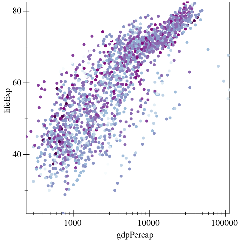
> (df-add-derived! gapminder "log-pop" '("pop") (λ (x) (log (first x) 10)))
> (graph #:data gapminder
         #:mapping (aes #:x "gdpPercap" #:y "lifeExp")
         #:x-transform logarithmic-transform
         #:legend-anchor 'no-legend
         #:theme theme-continuous
         (points #:mapping (aes #:continuous-color "log-pop")))

procedure
(theme->alist theme) → (listof (cons/c parameter? any/c))
theme : graphite-theme?

Converts a graphite-theme? to an association list of plot parameters to the values specified by the theme.

1	Graphing Procedures
2	Aesthetic Mappings
3	Renderers
4	Axis Transforms
5	Theming